Projected gradient descent - Mines Nancy

Again, consider the general constrained optimization problem

\begin{array}{ll} \minimize &\quad f_0(x)\\ \st &\quad x \in \Omega \end{array}

(1)

Goal: design a simple algorithm, based on first-order information $\nabla f$ to solve (1).

Recall from Chapter 4 that, for unconstrained problems ( $\Omega = \mathbb{R}^n$ ) with differentiable objective, one simple algorithm is gradient descent (GD):

x^{(k+1)} = x^{(k)}-\alpha_k\nabla f(x^{(k)}),\quad \alpha_k >0, \quad k=0, 1, \ldots

(2)

For constrained problems, a natural generalization is projected gradient descent (PGD), which combines GD with (Euclidean) projection onto $\Omega$ .

Projection onto a set¶

Comments

computing $P_{\Omega}(x_0)$ is itself an optimization problem
$P_{\Omega}(x_0)$ returns the closest point(s) (in Euclidean norm) to $x_0$ that belongs to the set $\Omega$
when $\Omega$ is closed and convex the projection is unique
if $x_0 \in \Omega$ , then $P_{\Omega}(x_0) = x_0$
in many important cases, $P_{\Omega}(x_0)$ can be computed explicitly. Example
$P_{\mathbb{R}_+^n}(x_0) = [\max(0, [x_0]_i)]_{i=1}^n \quad \text{ (entry-wise maximum)}$
(4)

Solution

Fix $x_0 \in \mathbb{R}^n$ . The optimization problem reads

\begin{array}{ll} \minimize& \quad \Vert x - x_0\Vert^2_2\\ \st &\quad \Vert x \Vert_2^2\leq 1 \end{array}

(5)

(We have used the fact that $\Vert x \Vert_2 \leq 1 \Leftrightarrow \Vert x \Vert_2^2 \leq 1$ , the latter being smooth in zero). This is a convex problem. Moreover Slater’s condition holds (the ball has a non-empty interior) so that strong duality holds. Therefore, KKT conditions are necessary and sufficient for optimality. One gets

\Vert \tilde{x}\Vert_2^2 \leq 1,\quad \lambda (\Vert\tilde{x}\Vert_2^2 -1) = 0,\quad \lambda \geq 0, \quad \tilde{x}-x_0 + \lambda \tilde{x} = 0

(6)

From stationarity of the Lagrangian we get $\tilde{x} = x_0/(1+\lambda)$ . Complementary slackness leads to two subcases:

$\lambda = 0$ . This implies $\tilde{x} = x_0$ , and by primal feasibilty $\Vert x_0 \Vert \leq 1$ .
$\lambda > 0$ . This implies $\Vert \tilde{x}\Vert_2 = 1$ . Hence $\Vert x_0/(1+\lambda)\Vert_2 =1$ which gives $\lambda = \Vert x_0\Vert_2-1$ . Hence $\tilde{x} = x_0 /\Vert x_0\Vert_2$ . Since $\lambda > 0$ by assumption, this case correspond to $\Vert x_0\Vert_2 > 1$ . Summarizing the results, we have
$P_\Omega(x_0) = \begin{cases} x_0& \quad \text{if } \Vert x_0 \Vert_2 \leq 1\\ x_0/\Vert x_0\Vert_2& \quad \text{ otherwise} \end{cases}$
(7)

Projected gradient algorithm¶

Typical step-size strategies

fixed-step size $\alpha_k = \alpha$ for all $k$
backtracking linesearch (determine $\alpha_k$ at each iteration based on sufficient decrease condition)

Example¶

Consider the optimization problem

\begin{split} \operatorname{minimize}&\quad (x_1-2)^2+(x_2-1)^2\\ \text{subject to}&\quad x_1^2 - x_2 \leq 0\\ &\quad x_1+x_2\leq 2 \end{split}

(8)

First, let us plot the objective function and feasible set.

import numpy as np
import matplotlib.pyplot as plt

# Objective function
def f(x, y):
    return (x - 2)**2 + (y - 1)**2

# Gradient
def dfdx(x, y):
    return np.array([2*(x - 2), 2*(y - 1)])

# Constraint boundaries
def c1(x):
    return x**2   # represents x^2 - y < 0
def c2(x):
    return 2 - x  # represents x + y < 2

# Ranges
xs = np.linspace(-5, 5, 400)
ys = np.linspace(-5, 5, 400)
X, Y = np.meshgrid(xs, ys)

# Prepare figure
plt.figure()

# Forbidden region from constraint 1: y < x^2
plt.fill_between(xs, c1(xs), ys.min(), color="gray", alpha=0.4,
                 label="Forbidden by constraint 1")

# Forbidden region from constraint 2: y > 2 - x
plt.fill_between(xs, c2(xs), ys.max(), color="gray", alpha=0.4,
                 label="Forbidden by constraint 2")

# Feasible region: x^2 < y < 2 - x
plt.fill_between(xs, c1(xs), c2(xs), where=c2(xs) > c1(xs),
                 color="green", alpha=0.2,
                 label="Feasible region")

# Contour of objective function
Z = f(X, Y)
plt.contour(X, Y, Z, cmap="inferno", levels=20)  # thermal-like colormap

# Global minimizer
plt.scatter([1], [1], s=40, label="Global minimizer (1,1)")

# Labels and limits
plt.xlabel("$x_1$")
plt.ylabel("$x_2$")
plt.xlim(-3, 2)
plt.ylim(-1, 5)
plt.legend()

plt.show()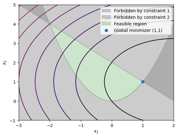

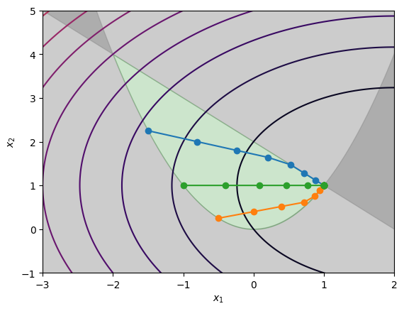
This can now visualize the trajectory of PGD for various starting points. In this example, we cannot compute easily the projection onto $\Omega$ , so that we compute it using a numerical solver (CVXPy, see in a few sections). The implementation is very basic, uses fixed step-size, and stops after a finite a number of iterations. Of course, we can do better, but that’s just to demonstrate how PGD forces iterates to be feasible by projecting the usual GD step onto $\Omega$ .

import numpy as np
import cvxpy as cp

# Projection onto the constraints
def projConstraints(x):
    z = cp.Variable(2)
    objective = cp.Minimize(cp.sum_squares(x - z))
    constraints = [
        z[0]**2 - z[1] <= 0,     # z1^2 - z2 <= 0
        z[0] + z[1] - 2 <= 0     # z1 + z2 <= 2
    ]
    problem = cp.Problem(objective, constraints)
    problem.solve(solver=cp.SCS, verbose=False)
    return z.value


# Projected Gradient Method
def ProjectedGradient(xinit, alpha, niter=10):
    xn = np.zeros((2, niter + 1))
    xn[:, 0] = xinit

    for n in range(niter):
        grad = dfdx(xn[0, n], xn[1, n])   # gradient at current iterate
        x_next = xn[:, n] - alpha * grad
        xn[:, n+1] = projConstraints(x_next)

    return xn

zn  = ProjectedGradient(np.array([-1.5, 1.5**2]), 0.1, niter=10)
zn2 = ProjectedGradient(np.array([-0.5, 0.5**2]), 0.1, niter=10)
zn3 = ProjectedGradient(np.array([-1.0, 1.0]), 0.1, niter=10)


# plotting

xs = np.linspace(-5, 5, 400)
ys = np.linspace(-5, 5, 400)
X, Y = np.meshgrid(xs, ys)

plt.figure()

# Forbidden regions
plt.fill_between(xs, c1(xs), ys.min(), color="gray", alpha=0.4)
plt.fill_between(xs, c2(xs), ys.max(), color="gray", alpha=0.4)

# Feasible region
plt.fill_between(xs, c1(xs), c2(xs), where=c2(xs) > c1(xs),
                 color="green", alpha=0.2)

# Objective contours
Z = f(X, Y)
plt.contour(X, Y, Z, cmap="inferno", levels=20)

# Trajectories
plt.plot(zn[0],  zn[1],  marker="o")
plt.plot(zn2[0], zn2[1], marker="o")
plt.plot(zn3[0], zn3[1], marker="o")

plt.xlim(-3, 2)
plt.ylim(-1, 5)
plt.xlabel("$x_1$")
plt.ylabel("$x_2$")

8.2 Projected gradient descent

Projection onto a set¶

Projected gradient algorithm¶

Example¶

Comments on projected gradient descent¶