8.3 Uzawa’s method
We now move to a different kind of algorithm, which exploits duality . The main idea of Uzawa’s method is to apply the projected gradient method to the dual problem.
First let us start with a reminder from Chapter 7 . The primal problem we consider has the form
minimize f 0 ( x ) subject to f i ( x ) ≤ 0 , i = 1 , … , m h i ( x ) = 0 , i = 1 , … , p \begin{split}
\minimize&\quad f_0(x)\\
\text{subject to}&\quad f_i(x) \leq 0, \quad i = 1, \ldots, m\\
&\quad h_i(x) = 0, \quad i = 1, \ldots, p
\end{split} minimize subject to f 0 ( x ) f i ( x ) ≤ 0 , i = 1 , … , m h i ( x ) = 0 , i = 1 , … , p and the associated dual problem is
maximize g ( λ , ν ) : = inf x ∈ D L ( x , λ , ν ) subject to λ ≥ 0 \begin{split}
\maximize&\quad g({\lambda}, {\nu}):= \inf_{x\in \mathcal{D}} L(x, {\lambda}, {\nu})\\
\text{subject to}&\quad {\lambda} \geq 0
\end{split} maximize subject to g ( λ , ν ) := x ∈ D inf L ( x , λ , ν ) λ ≥ 0 where L L L
L ( x , λ , ν ) = f 0 ( x ) + ∑ i = 1 m λ i f i ( x ) + ∑ i = 1 p ν i h i ( x ) L(x, {\lambda}, {\nu}) = f_0(x) + \sum_{i=1}^m\lambda_i f_i(x) + \sum_{i=1}^p \nu_i h_i(x) L ( x , λ , ν ) = f 0 ( x ) + i = 1 ∑ m λ i f i ( x ) + i = 1 ∑ p ν i h i ( x ) Principle ¶ The dual problem is a constrained optimization problem with non-negativity constraints λ ≥ 0 \lambda \geq 0 λ ≥ 0 explicit and efficient :
P R + m ( λ ) = [ max ( 0 , λ i ) ] i = 1 m P_{\mathbb{R}_+^m}(\lambda) = [\max(0, \lambda_i)]_{i=1}^m P R + m ( λ ) = [ max ( 0 , λ i ) ] i = 1 m Since the dual problem is a maximization problem, we can use projected gradient ascent on the Lagrangian L ( x ( k ) , λ , ν ) L(x^{(k)}, \lambda, \nu) L ( x ( k ) , λ , ν ) x ( k ) x^{(k)} x ( k )
given current ( λ ( k ) , ν ( k ) ) (\lambda^{(k)}, \nu^{(k)}) ( λ ( k ) , ν ( k ) ) x ( k + 1 ) ∈ arg min L ( x , λ ( k ) , ν ( k ) ) ) x^{(k+1)} \in \argmin L(x, \lambda^{(k)}, \nu^{(k)})) x ( k + 1 ) ∈ arg min L ( x , λ ( k ) , ν ( k ) ))
then update the Lagrange multipliers by a step of gradient ascent. Since the Lagrangian is separable in ( λ , ν ) (\lambda, \nu) ( λ , ν )
λ i ( k + 1 ) = max ( 0 , λ i ( k ) + α k f i ( x ( k + 1 ) ) ) \lambda^{(k+1)}_i = \max(0, \lambda^{(k)}_i + \alpha_k f_i(x^{(k+1)})) λ i ( k + 1 ) = max ( 0 , λ i ( k ) + α k f i ( x ( k + 1 ) )) i = 1 , … , m i=1, \ldots, m i = 1 , … , m
ν i ( k + 1 ) = ν i ( k ) + β k h i ( x ( k + 1 ) ) \nu^{(k+1)}_i =\nu^{(k)}_i + \beta_k h_i(x^{(k+1)}) ν i ( k + 1 ) = ν i ( k ) + β k h i ( x ( k + 1 ) ) i = 1 , … , p i=1, \ldots, p i = 1 , … , p
and so on until convergence.
Under suitable conditions, such algorithm is shown to converge to a saddle-point of the Lagrangian (hence it yields primal and dual optimal points).
input : initial λ ( 0 ) , ν ( 0 ) \lambda^{(0)}, \nu^{(0)} λ ( 0 ) , ν ( 0 )
k:=0
while stopping criterion not satisfied do
Primal update x ( k + 1 ) ∈ arg min L ( x , λ ( k ) , ν ( k ) ) ) x^{(k+1)} \in \argmin L(x, \lambda^{(k)}, \nu^{(k)})) x ( k + 1 ) ∈ arg min L ( x , λ ( k ) , ν ( k ) ))
Dual ascent
λ i ( k + 1 ) = max ( 0 , λ i ( k ) + α k f i ( x ( k + 1 ) ) ) \lambda^{(k+1)}_i = \max(0, \lambda^{(k)}_i + \alpha_k f_i(x^{(k+1)})) λ i ( k + 1 ) = max ( 0 , λ i ( k ) + α k f i ( x ( k + 1 ) )) i = 1 , … , m i=1, \ldots, m i = 1 , … , m
ν i ( k + 1 ) = ν i ( k ) + β k h i ( x ( k + 1 ) ) \nu^{(k+1)}_i =\nu^{(k)}_i + \beta_k h_i(x^{(k+1)}) ν i ( k + 1 ) = ν i ( k ) + β k h i ( x ( k + 1 ) ) i = 1 , … , p i=1, \ldots, p i = 1 , … , p
k:=k+1
return aproximate solution x ( k ) x^{(k)} x ( k )
Examples ¶ 1D example ¶ Consider the following problem
minimize x 2 subject to ( x − 2 ) ( x − 4 ) ≤ 0 \begin{split}
\minimize&\quad x^2\\
\text{subject to}&\quad (x-2)(x-4)\leq 0
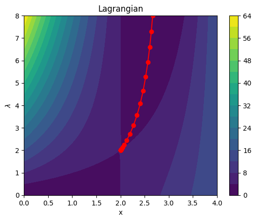
\end{split} minimize subject to x 2 ( x − 2 ) ( x − 4 ) ≤ 0 with trivial solution x ⋆ = 2 x^\star = 2 x ⋆ = 2 L ( x , λ ) = x 2 + λ ( x − 2 ) ( x − 4 ) = ( 1 + λ ) x 2 − 6 λ + 8 L(x, \lambda) = x^2+ \lambda (x-2)(x-4) = (1+\lambda)x^2 -6\lambda + 8 L ( x , λ ) = x 2 + λ ( x − 2 ) ( x − 4 ) = ( 1 + λ ) x 2 − 6 λ + 8
For fixed λ ≥ 0 \lambda \geq 0 λ ≥ 0 arg min x L ( x , λ ) = 3 λ / ( 1 + λ ) \argmin_x L(x, \lambda) = 3\lambda/(1+\lambda) arg min x L ( x , λ ) = 3 λ / ( 1 + λ ) α k = α \alpha_k = \alpha α k = α
x ( k + 1 ) : = 3 λ ( k ) / ( 1 + λ ( k ) ) λ ( k + 1 ) : = max ( 0 , λ k + α ( x ( k + 1 ) − 2 ) ( x ( k + 1 ) − 4 ) ) \begin{align}
x^{(k+1)} &:= 3\lambda^{(k)}/(1+\lambda^{(k)})\\
\lambda^{(k+1)} &:= \max(0, \lambda^{k} + \alpha (x^{(k+1)} - 2)(x^{(k+1)} - 4))
\end{align} x ( k + 1 ) λ ( k + 1 ) := 3 λ ( k ) / ( 1 + λ ( k ) ) := max ( 0 , λ k + α ( x ( k + 1 ) − 2 ) ( x ( k + 1 ) − 4 )) and so on, until convergence. Here’s a small example of trajectory on the Lagrangian, for λ ( 0 ) = 8 \lambda^{(0)} = 8 λ ( 0 ) = 8
import numpy as np
import matplotlib.pyplot as plt

def f0(x):
    return x**2

def f1(x):
    return (x-2)*(x-4)

def L(x, l):
    return f0(x) + l*f1(x)

def uzawa(l0, alpha=0.1, niter=10):


    lks = [l0]
    xks = []
    for k in range(niter):
        xks.append(3*lks[k]/(1+lks[k]))
        lk1 = np.maximum(0, lks[k]+ alpha*f1(xks[-1]))
        lks.append(lk1)
    return xks, lks

xks, lks = uzawa(8, alpha=.8, niter=50)
x = np.linspace(0, 4)
l = np.linspace(0, 8)
xx, ll = np.meshgrid(x, l)

plt.contourf(x, l, L(xx,ll), levels=20)
plt.xlabel('x')
plt.ylabel('$\lambda$')
plt.colorbar()
plt.title('Lagrangian')

plt.plot(xks, lks[:-1], '-o', c='r', )
We clearly observe converge to the optimums λ ⋆ = 2 \lambda^\star = 2 λ ⋆ = 2 x ⋆ = 2 x^\star = 2 x ⋆ = 2
Non-negative least squares ¶ Let us write Uzawa’s iterates for the following problem
minimize 1 2 ∥ y − A x ∥ 2 2 subject to x ≥ 0 \begin{split}
\minimize&\quad \frac{1}{2}\Vert y - Ax\Vert_2^2\\
\text{subject to}&\quad x\geq 0
\end{split} minimize subject to 2 1 ∥ y − A x ∥ 2 2 x ≥ 0 where A A A
The Lagrangian for the problem is L ( x , λ ) = 1 2 ∥ y − A x ∥ 2 2 − λ ⊤ x L(x, {\lambda}) = \frac{1}{2}\Vert y - Ax\Vert_2^2 - {\lambda}^\top x L ( x , λ ) = 2 1 ∥ y − A x ∥ 2 2 − λ ⊤ x x x x ∇ x L ( x , λ ) = A ⊤ ( A x − y ) − λ \nabla_{x} L(x, {\lambda}) = A^\top (Ax-y) -{\lambda} ∇ x L ( x , λ ) = A ⊤ ( A x − y ) − λ
x ( k + 1 ) = ( A ⊤ A ) − 1 [ A ⊤ y + λ ( k ) ] λ ( k + 1 ) = [ λ ( k ) − α k x ( k + 1 ) ] + \begin{align*}
x^{(k+1)} = (A^\top A)^{-1}\left[A^\top y + {\lambda}^{(k)}\right]\\
{\lambda}^{(k+1)} =[{\lambda}^{(k)} -\alpha_k x^{(k+1)}]^+
\end{align*} x ( k + 1 ) = ( A ⊤ A ) − 1 [ A ⊤ y + λ ( k ) ] λ ( k + 1 ) = [ λ ( k ) − α k x ( k + 1 ) ] + until primal and dual convergence.