Let us recall the (unconstrained) optimization problem at hand
The gradient descent method attempts at solving (1) using the following algorihtm.
Under suitable assumptions about the objective , and proper choice of the stepsize at each iteration, one can show that the sequence of iterates produced by gradient descent converges to a stationary point of the cost function. We’ll cover in more detail in Chapter 5.
Step-size selection strategies¶
Choosing an appropriate step-size is crucial for the efficiency and convergence of gradient descent. The step-size determines how far each iteration moves towards a (local) minimum, and poor choices can lead to slow progress or even divergence.
Constant step-size¶
This first choice is also the simplest (and still used in many situations).
Intuitively, the stepsize should be chosen as a compromise between the rate of convergence and convergence guarantees. Indeed if is “too small” then convergence of the algorithm will be very slow; on the contrary if is chosen “too large”, then there exist a risk of divergence of the algorithm.
A glimpse at convergence guarantees
We’ll cover this in more detail in Chapter 5, but here is a first result. Let be differentiable with -Lipschitz gradient, i.e.,
and let be bounded below, i.e. for all , . Then, if
then the gradient descent method generates iterates with
i.e., gradient descent generates a sequence of non-increasing objective values which identifies a stationary point of the objective.
Optimal step-size (exact line search)¶
This strategy guarantees the best decrease of the objective for the current descent direction . However, a major drawback is that calculating the optimal step size can be as difficult as the original problem and/or very computationally expensive.
Example 1 (adapted from Boyd & Vandenberghe (2004, §9.3.2))
Backtracking line search¶
This last strategy searches a step size that sufficiently decreases the objective at each iteration, i.e., such that where is some (negative) constant. Backtracking is the most commonly used approach in practice, for which many ``recipes’’ for the choice of exist.
In this course, we will focus on a standard condition known as Armijo’s condition (also simply referred to as backtracking linesearch condition). In the case of gradient descent, this condition requires that the stepsize sufficiently decreases the cost function such that
where is a parameter of the method.
Illustration The following code snippets show how backtracking iteratively “test” step sizes until the sufficient decrease condition is satisfied.
Source
import numpy as np
import matplotlib.pyplot as plt

# Define function and gradient
def f(x):
    return x**2

def dfdx(x):
    return 2*x

# Starting point
xk = -1

# Define line cost and linear approximation
def linCost(t):
    return f(xk - t * dfdx(xk))

def linApp(t):
    return f(xk) - t * (dfdx(xk)**2)

# Range of step sizes
ts = np.linspace(0, 1, 200)

# Parameter combinations
params = [(0.2, 0.6), (0.05, 0.6), (0.2, 0.95), (0.05, 0.95)]

fig, axes = plt.subplots(2, 2, figsize=(14, 10))

for ax, (s, eta) in zip(axes.ravel(), params):
    alpha_0 = 1.0
    nbck = 0

    # Plot curves
    ax.plot(ts, linCost(ts), label=r"$f(x^{(k)} - \alpha \nabla f(x^{(k)}))$", linewidth=2)
    ax.plot(ts, linApp(s*ts), label=r"$f(x^{(k)}) - s \alpha \|\nabla f(x^{(k)})\|^2$", linewidth=2)

    # Backtracking loop
    while linCost(alpha_0) > linApp(s*alpha_0):
        ax.annotate(f"iter {nbck}",
                    xy=(alpha_0, linCost(alpha_0)),
                    xytext=(alpha_0+0.05, linCost(alpha_0)),
                    arrowprops=dict(arrowstyle="->", color="gray"),
                    fontsize=9, color="black", backgroundcolor="w")
        ax.scatter([alpha_0], [linCost(alpha_0)], color="blue")
        ax.scatter([alpha_0], [linApp(s*alpha_0)], color="red")
        ax.axvline(x=alpha_0, linestyle="--", color="black")
        alpha_0 = eta * alpha_0
        nbck += 1

    # Final accepted step
    ax.annotate(f"iter {nbck}",
                xy=(alpha_0, linCost(alpha_0)),
                xytext=(alpha_0+0.05, linCost(alpha_0)),
                arrowprops=dict(arrowstyle="->", color="gray"),
                fontsize=9, color="black", backgroundcolor="w")
    ax.scatter([alpha_0], [linCost(alpha_0)], color="blue", zorder=5)
    ax.scatter([alpha_0], [linApp(s*alpha_0)], color="red", zorder=5)
    ax.axvline(x=alpha_0, linestyle="--", color="black")

    # Labels and titles
    ax.set_xlabel(r"$\alpha$")
    ax.set_title(f"Backtracking LS (s={s}, η={eta})")
    ax.grid(True)
    ax.legend(fontsize=8)

plt.tight_layout()
plt.show()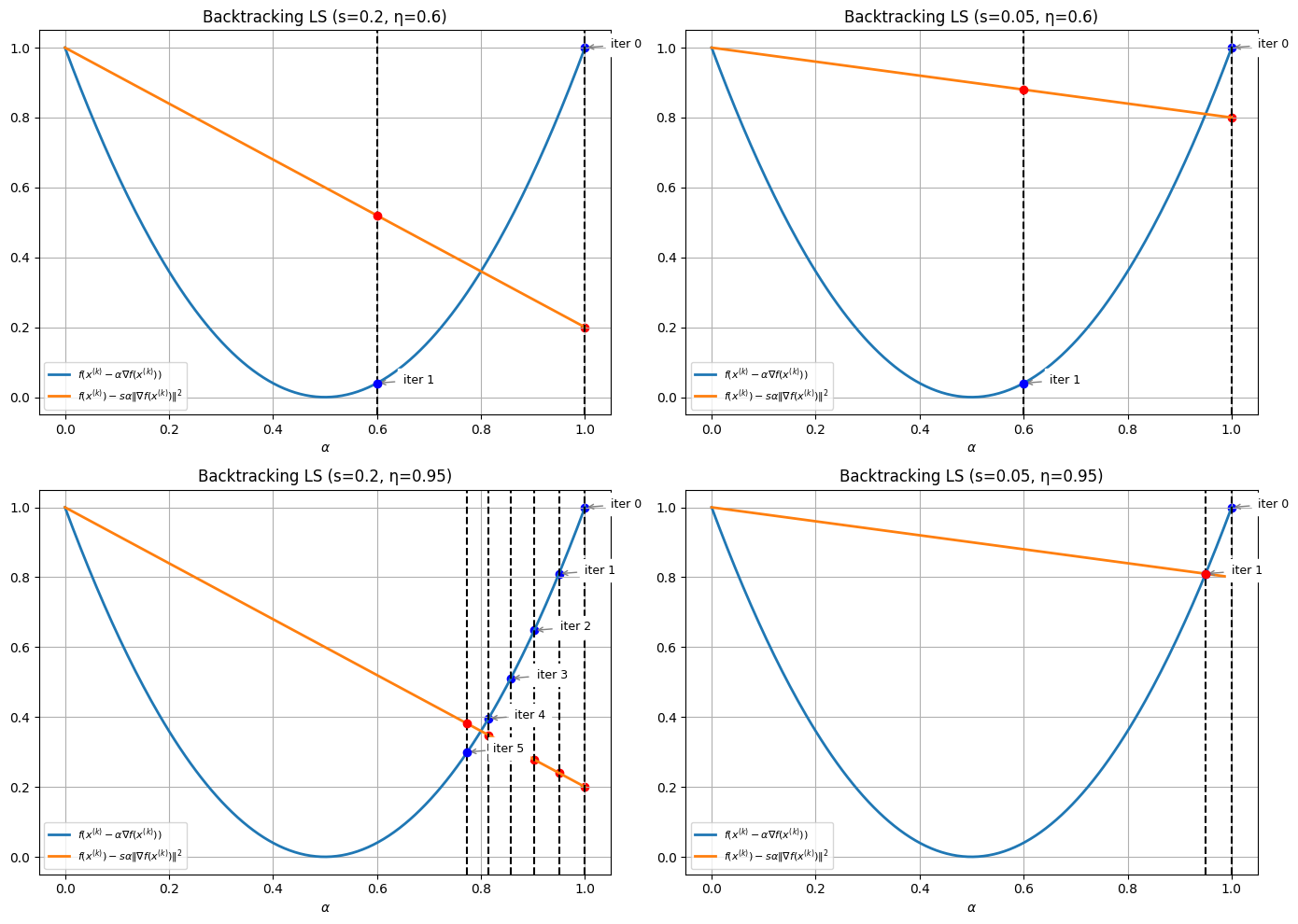
In a nutshell:
controls the tightness of the sufficient decrease condition: the closer is to 0, the easier it is to satisfy the condition
controls the gaps between successive candidate steps: the closer is to 1, the slower the algorithm, but also the closer will be of the minimal stepsize that satisfies the decrease condition.
in practice, one has to chose to maintain a good trade-off between convergence rate and computational cost.
Comparison of step-size strategies¶
To compare the effect of the proposed step-size selection strategies, let us consider the following example, adapted from Boyd & Vandenberghe (2004).
Let us plot the objective.
import numpy as np
import matplotlib.pyplot as plt

def f(x1, x2):
    return np.exp(x1 +3*x2 - 0.1) + np.exp(x1 -3*x2- 0.1) + np.exp(-x1 - 0.1)


x1s = np.linspace(-2, 0.6, 50)
x2s = np.linspace(-0.5, 0.5, 50)
X1, X2 = np.meshgrid(x1s, x2s)
Z = f(X1, X2)

plt.figure(figsize=(8, 6))
cp = plt.contourf(X1, X2, Z, levels=30, cmap='viridis')
plt.colorbar(cp)
plt.xlabel("$x_1$")
plt.ylabel("$x_2$")
plt.title("$f_0$")
plt.show()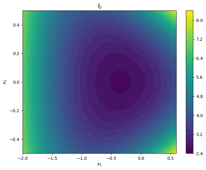
We will now compare the three step-sizes: fixed, optimal, and with backtracking. For simplicity, we only implemented a fixed number of iterations; recall that in practice you need a good stopping criterion!
In addition, we will a backtracking strategy in which the value of is not reset to at each iteration; this is used in some context to save some computation time. You can see the effect by uncommenting this line in the code.
Source
from scipy.optimize import minimize_scalar, minimize

def dfdx(x1, x2):
    dx1 = np.exp(x1 + 3*x2 - 0.1) + np.exp(x1 - 3*x2 - 0.1) - np.exp(-x1 - 0.1)
    dx2 = 3 * np.exp(x1 + 3*x2 - 0.1) - 3 * np.exp(x1 - 3*x2 - 0.1)
    return np.array([dx1, dx2])


# Initial point
x0 = np.array([-2, 0.5])
max_iter = 25

# Fixed step-size
alpha_fixed = 0.1
xs_fixed = [x0.copy()]
for _ in range(max_iter):
    grad = dfdx(*xs_fixed[-1])
    xs_fixed.append(xs_fixed[-1] - alpha_fixed * grad)

# Optimal step-size (exact line search)
xs_opt = [x0.copy()]
for _ in range(max_iter):
    grad = dfdx(*xs_opt[-1])
    # Line search: minimize f(x - alpha * grad) over alpha >= 0
    def phi(alpha):
        return f(*(xs_opt[-1] - alpha * grad))
    res = minimize_scalar(phi)
    alpha_opt = res.x
    xs_opt.append(xs_opt[-1] - alpha_opt * grad)

# Backtracking line search
s = 0.3
eta = 0.9
alpha0 = .2
xs_bt = [x0.copy()]
alpha = alpha0
for n in range(max_iter):
    grad = dfdx(*xs_bt[-1])
    #alpha = alpha0 # uncomment if you want to reset alpha = alpha0 at each iteration
    while f(*(xs_bt[-1] - alpha * grad)) > f(*xs_bt[-1]) - s * alpha * np.linalg.norm(grad)**2:
        alpha *= eta
        print(f'backtracking kicks in at iter {n}: current alpha = {alpha}')
    xs_bt.append(xs_bt[-1] - alpha * grad)

# Plot trajectories
plt.figure(figsize=(8, 6))
cp = plt.contourf(X1, X2, Z, levels=30, cmap='viridis')
plt.contour(X1, X2, Z, levels=30)
plt.colorbar(cp)
plt.xlabel("$x_1$")
plt.ylabel("$x_2$")
plt.title("Gradient Descent Trajectories")

def plot_path(xs, label):
    xs = np.array(xs)
    plt.plot(xs[:,0], xs[:,1], marker='o', label=label)

plot_path(xs_fixed, r"Fixed step-size $\alpha$" + f"$= {alpha_fixed}$")
plot_path(xs_opt, "Optimal step-size")
plot_path(xs_bt, f"Backtracking $(s, \eta) = {s, eta}$")
plt.legend()
plt.show()

# compute optimal value
res = minimize(lambda x: f(x[0], x[1]), x0)
pstar = res.fun

# Plot objective values for each method
plt.figure(figsize=(8, 6))
plt.semilogy([f(*x) - pstar for x in xs_fixed], label=r"Fixed step-size $\alpha$" + f"$= {alpha_fixed}$", marker='o')
plt.semilogy([f(*x)- pstar for x in xs_opt], label="Optimal step-size", marker='o')
plt.semilogy([f(*x)- pstar for x in xs_bt], label=f"Backtracking $(s, \eta) = {s, eta}$", marker='o')
plt.xlabel("Iteration")
plt.ylabel("$f_0(x) - p^\star$")
plt.title("suboptimality value vs iteration")
plt.legend()
plt.grid(True)
plt.show()
backtracking kicks in at iter 2: current alpha = 0.18000000000000002
backtracking kicks in at iter 3: current alpha = 0.16200000000000003
backtracking kicks in at iter 3: current alpha = 0.14580000000000004
backtracking kicks in at iter 13: current alpha = 0.13122000000000003
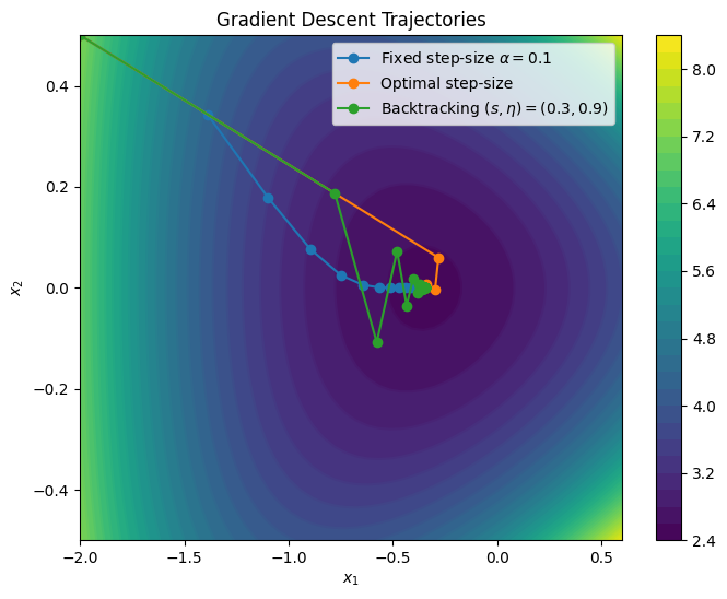
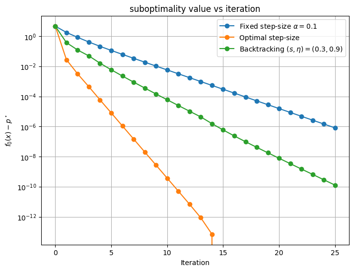
This experiment shows that among the three methods, the simpler (fixed-step size) is also the slowest. Both backtracking and optimal step size converge faster, with an advantage to the optimal step-size strategy for this configuration. However, this is not always the case: there are situations in which backtracking can outperform (sometimes in a striking way) the optimal step-size strategy.
Here is an example, starting from a different point and with updated parameters. (note we reset in each iteration).
Source
# Initial point
x0 = np.array([.5, .5])
max_iter = 25

# Fixed step-size
alpha_fixed = 0.03
xs_fixed = [x0.copy()]
for _ in range(max_iter):
    grad = dfdx(*xs_fixed[-1])
    xs_fixed.append(xs_fixed[-1] - alpha_fixed * grad)

# Optimal step-size (exact line search)
xs_opt = [x0.copy()]
for _ in range(max_iter):
    grad = dfdx(*xs_opt[-1])
    # Line search: minimize f(x - alpha * grad) over alpha >= 0
    def phi(alpha):
        return f(*(xs_opt[-1] - alpha * grad))
    res = minimize_scalar(phi)
    alpha_opt = res.x
    xs_opt.append(xs_opt[-1] - alpha_opt * grad)

# Backtracking line search
s = 0.1
eta = 0.3
alpha0 = 1
xs_bt = [x0.copy()]
alpha = alpha0
for n in range(max_iter):
    grad = dfdx(*xs_bt[-1])
    alpha = alpha0 # uncomment if you want to reset alpha = alpha0 at each iteration
    while f(*(xs_bt[-1] - alpha * grad)) > f(*xs_bt[-1]) - s * alpha * np.linalg.norm(grad)**2:
        alpha *= eta
        print(f'backtracking kicks in at iter {n}: current alpha = {alpha}')
    xs_bt.append(xs_bt[-1] - alpha * grad)

# Plot trajectories
plt.figure(figsize=(8, 6))
cp = plt.contourf(X1, X2, Z, levels=30, cmap='viridis')
plt.contour(X1, X2, Z, levels=30)
plt.colorbar(cp)
plt.xlabel("$x_1$")
plt.ylabel("$x_2$")
plt.title("Gradient Descent Trajectories")

def plot_path(xs, label):
    xs = np.array(xs)
    plt.plot(xs[:,0], xs[:,1], marker='o', label=label)

plot_path(xs_fixed, r"Fixed step-size $\alpha$" + f"$= {alpha_fixed}$")
plot_path(xs_opt, "Optimal step-size")
plot_path(xs_bt, f"Backtracking $(s, \eta) = {s, eta}$")
plt.legend()
plt.show()

# compute optimal value
res = minimize(lambda x: f(x[0], x[1]), x0)
pstar = res.fun

# Plot objective values for each method
plt.figure(figsize=(8, 6))
plt.semilogy([f(*x) - pstar for x in xs_fixed], label=r"Fixed step-size $\alpha$" + f"$= {alpha_fixed}$", marker='o')
plt.semilogy([f(*x)- pstar for x in xs_opt], label="Optimal step-size", marker='o')
plt.semilogy([f(*x)- pstar for x in xs_bt], label=f"Backtracking $(s, \eta) = {s, eta}$", marker='o')
plt.xlabel("Iteration")
plt.ylabel("$f_0(x) - p^\star$")
plt.title("suboptimality value vs iteration")
plt.legend()
plt.grid(True)
plt.show()
backtracking kicks in at iter 0: current alpha = 0.3
backtracking kicks in at iter 0: current alpha = 0.09
backtracking kicks in at iter 0: current alpha = 0.027
backtracking kicks in at iter 1: current alpha = 0.3
backtracking kicks in at iter 2: current alpha = 0.3
backtracking kicks in at iter 2: current alpha = 0.09
backtracking kicks in at iter 3: current alpha = 0.3
backtracking kicks in at iter 3: current alpha = 0.09
backtracking kicks in at iter 4: current alpha = 0.3
backtracking kicks in at iter 5: current alpha = 0.3
backtracking kicks in at iter 5: current alpha = 0.09
backtracking kicks in at iter 6: current alpha = 0.3
backtracking kicks in at iter 7: current alpha = 0.3
backtracking kicks in at iter 7: current alpha = 0.09
backtracking kicks in at iter 8: current alpha = 0.3
backtracking kicks in at iter 9: current alpha = 0.3
backtracking kicks in at iter 10: current alpha = 0.3
backtracking kicks in at iter 10: current alpha = 0.09
backtracking kicks in at iter 11: current alpha = 0.3
backtracking kicks in at iter 12: current alpha = 0.3
backtracking kicks in at iter 12: current alpha = 0.09
backtracking kicks in at iter 13: current alpha = 0.3
backtracking kicks in at iter 14: current alpha = 0.3
backtracking kicks in at iter 14: current alpha = 0.09
backtracking kicks in at iter 15: current alpha = 0.3
backtracking kicks in at iter 16: current alpha = 0.3
backtracking kicks in at iter 16: current alpha = 0.09
backtracking kicks in at iter 17: current alpha = 0.3
backtracking kicks in at iter 18: current alpha = 0.3
backtracking kicks in at iter 19: current alpha = 0.3
backtracking kicks in at iter 19: current alpha = 0.09
backtracking kicks in at iter 20: current alpha = 0.3
backtracking kicks in at iter 21: current alpha = 0.3
backtracking kicks in at iter 22: current alpha = 0.3
backtracking kicks in at iter 22: current alpha = 0.09
backtracking kicks in at iter 24: current alpha = 0.3
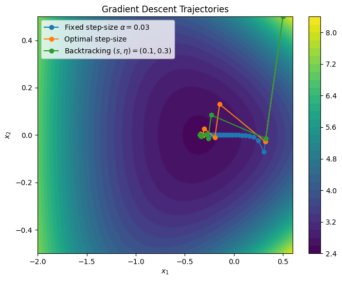
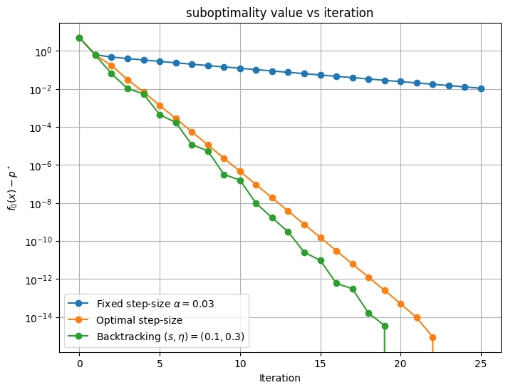
In this example backtracking outperforms the optimal step-size strategy; it is less prone to zig-zags, and thus converges faster. Both methods converge faster than the fixed step-size strategy.
Takeaway: step-size selection strategies¶
- Boyd, S. P., & Vandenberghe, L. (2004). Convex optimization. Cambridge University Press.