8.1 Penalty method

Principle¶

Consider the optimization problem

where $f_0$ is the objective and $\Omega \subset \mathbb{R}^n$ is the constraint set.

Key idea : replace (1) with the unconstrained optimization problem

where $p:\mathbb{R}^n \rightarrow \mathbb{R}$ is the penalty function such that

• $p$ is continuous

• $p(x) > 0$ if $x \notin \Omega$

• $p(x) = 0$ if $x \in \Omega$.

The penalty parameter $\rho$ controls the cost of violating the constraints.

Choosing penalty functions¶

Recall $\Omega$ is often parameterized by equality and inequality constraints.

Typical choices of penalty functions: use \alert{quadratic functions}

• inequality constraint $f_i(x) \leq 0$: take

  $$p(x) = \frac{1}{2}\left[\max(0, f_i(x))\right]^2 := \frac{1}{2}\left[f_i^+(x)\right]^2$$

  (4)

• equality constraint $h_i(x) = 0$: take

  $$p(x) = \frac{1}{2} (h_i(x))^2$$

  (5)

  For multiple constraints, we simply sum all individual penalties. For $\Omega$ defined in (3) one would get

  $$p(x) = \frac{1}{2}\sum_{i=1}^m (f_i^+(x))^2 + \frac{1}{2}\sum_{i=1}^p (h_i(x))^2$$

  (6)

Note that besides quadratic functions, one can consider also non-smooth penalties such as $\ell_1$-norm with very interesting properties (outside the scope of this lecture).

Penalty method algorithm¶

We thus replace solving (1) by solving a succession of unconstrained penalized problems

with increasing penalties $\rho_1 < \rho_2 < \ldots < \rho_k \rightarrow +\infty$.

This results suggests the following algorithm.

How-to compute solutions of penalized problems?¶

Consider a problem with one inequality constraint $f_1(x) \le 0$. The quadratic penalty is

How to compute the gradient of the penalty function?

A potential concern is that $f_1^+$ is not differentiable at points where $f_1(x)=0$. However, the penalty can be written as a composition

Although the map $y\mapsto \max(0,y)$ is not differentiable at 0, the quadratic penalty $\gamma$ is differentiable everywhere, because

and in particular $\gamma'(0)=0$. Therefore, if $f_1$ is differentiable, the chain rule applies.

Using the chain rule,

Thus the quadratic penalty is differentiable (but not twice differentiable) even at points where the constraint is active, and its gradient is given by the expression above.

Examples¶

A simple problem¶

Consider the (very) simple problem

and solve it using the penalty method.

Minimum-norm solution of linear equations¶

Using the penalty method, solve the following problem:

A nonconvex 1D example¶

We consider the following nonconvex optimization problem

The feasible set of this problem is nonconvex, as shown by the plot below (green area).

Source

import numpy as np
import matplotlib.pyplot as plt

# define objective and constraints
def f(x, y):
    return (x - 2)**2 + (y + 1)**2

def g(x, y):
    """Nonlinear inequality constraint g(x,y) <= 0"""
    return -(2- x**2-y**2 +  np.sin(3*x) * np.cos(2*y))

# Grid for contour plots
xx = np.linspace(-2.5, 3, 400)
yy = np.linspace(-2.5, 2.5, 400)
X, Y = np.meshgrid(xx, yy)

F = f(X, Y)
G = g(X, Y)

plt.figure(figsize=(10, 8))

# Objective contours
CS1 = plt.contour(X, Y, F, levels=20, cmap='viridis', alpha=0.6)
plt.clabel(CS1, inline=1, fontsize=8)

# Constraint boundary (g(x,y)=0)
CS2 = plt.contour(X, Y, G, levels=[0], colors='red', linewidths=2)
plt.clabel(CS2, fmt={0: '$f_1(x) = 0$'}, fontsize=10)

# Feasible region shading
plt.contourf(X, Y, G, levels=[-10, 0], colors=['#d0ffd0'], alpha=0.3)
plt.xlabel("$x_1$")
plt.ylabel("$x_2$")
plt.scatter(2, -1, color='black', marker='*', s=150, label='Unconstrained solution')
plt.legend()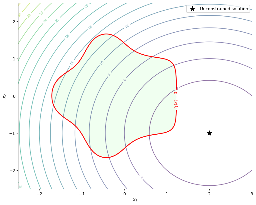

Let us display how the penalized cost function will look for different values of $\rho$.

Source

rhos = [0, .1, .5, 1]
Gplus = np.maximum(0, G)
fig, ax = plt.subplots(ncols=len(rhos), figsize=(12, 4), sharex=True, sharey=True)
for i, rho in enumerate(rhos):

    ax[i].contour(X, Y, F+rho*(Gplus)**2)
    ax[i].set_title(r'$\rho = '+str(rho)+'$')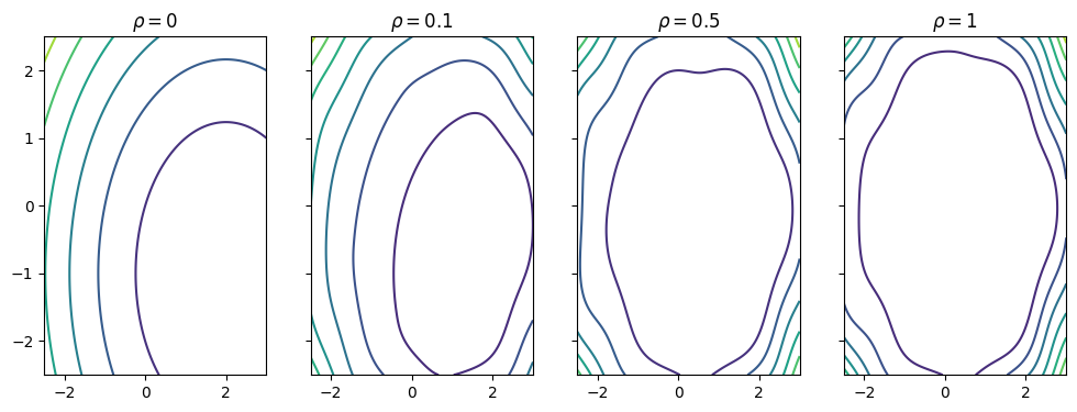

We can iteratively minimize penalized problems with increasing penalty parameter $\rho$. Let’s do this numerically and plot the results.

Source

# redefine function to be used with scipy minimize
from scipy.optimize import minimize

def f(xy):
    x, y = xy
    return (x - 2)**2 + (y + 1)**2

def g(xy):
    x, y = xy
    return -(2- x**2-y**2 +  np.sin(3*x) * np.cos(2*y))

def g_plus(xy):
    return max(0.0, g(xy))

# penalized objective
def P_mu(xy, rho):
    return f(xy) + 0.5 * rho * g_plus(xy)**2


rhos = [1, 2, 5, 10, 100]
solutions = []

x0 = np.array([2, -1])   # initial guess

for rho in rhos:

    # Wrap for minimize
    fun = lambda xy: P_mu(xy, rho)

    # Run optimizer
    res = minimize(fun, x0, method='BFGS') #options={'disp': True} to show details

    sol = res.x
    solutions.append(sol)


    # warm start next iteration
    x0 = sol

print("\nSolutions for increasing rho:")
for rho, sol in zip(rhos, solutions):
    print(f"rho={rho:4d}:  x={sol},  f_1(x)={g(sol)}")

## plots
xx = np.linspace(-2.5, 3, 400)
yy = np.linspace(-2.5, 2.5, 400)
X, Y = np.meshgrid(xx, yy)

F = (X - 2)**2 + (Y + 1)**2
G = X**2+Y**2 -  np.sin(3*X) * np.cos(2*Y)-2

plt.figure(figsize=(10, 8))

# Objective contours
CS1 = plt.contour(X, Y, F, levels=20, cmap='viridis', alpha=0.6)
plt.clabel(CS1, inline=1, fontsize=8)

# Constraint boundary
CS2 = plt.contour(X, Y, G, levels=[0], colors='red', linewidths=2)
plt.clabel(CS2, fmt={0: "$f_1(x) = 0$"}, fontsize=10)

# Feasible region shading
plt.contourf(X, Y, G, levels=[-10, 0], colors=['#d0ffd0'], alpha=0.3)

# Plot solutions for each mu
colors = ['blue', 'green', 'orange', 'purple', 'red']
for sol, rho, col in zip(solutions, rhos, colors):
    plt.scatter(sol[0], sol[1], color=col, s=80, label=f"ρ={rho}")


plt.title("Penalty Method in 2D")
plt.xlabel("$x_1$")
plt.ylabel("$x_2$")
plt.scatter(2, -1, color='black', marker='*', s=150, label='Unconstrained solution')
plt.legend()
plt.grid(alpha=0.3)
plt.show()

Solutions for increasing rho:
rho=   1:  x=[ 1.38285633 -0.93313364],  f_1(x)=0.5369100930598791
rho=   2:  x=[ 1.29431356 -0.86992303],  f_1(x)=0.3184002494305595
rho=   5:  x=[ 1.22615353 -0.8057165 ],  f_1(x)=0.13185377660643813
rho=  10:  x=[ 1.20427496 -0.78335207],  f_1(x)=0.06577643106933301
rho= 100:  x=[ 1.18560937 -0.76388718],  f_1(x)=0.006543126703541777

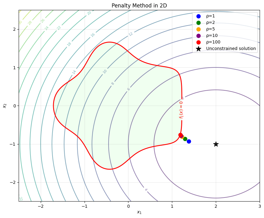
In the limit of large $\rho$, we would get the (unique) solution to the initial problem. Stopping at a given $\rho$ value gives an approximation of that point, characterized by the value of $f_1(x)$, which quantifies “how much” we are violating the constraint.