Nonlinear conjugate gradient methods - Mines Nancy

Motivation¶

The linear conjugate gradient method provides an iterative solution to the linear system $Qx = p$ , or equivalently, a solution to the corresponding quadratic program

\begin{array}{ll} \minimize& f_0(x):=\frac{1}{2} x^\top Q x - p^\top x\\ \st & x \in \mathbb{R}^n \end{array}\quad \quad Q \succ 0

(1)

Nonlinear conjugate gradient methods extend the ideas of linear conjugate gradient to non-quadratic objective functions $f_0$ . Several variant exists, two popular ones being

the Fletcher-Reeves meethod (FR)
the Polak-Ribière method (PR)

The key principle is the following: replace the residual $r_k$ (which is the gradient of quadratic $f_0$ ) by the evaluation of the gradient of the nonlinear objective $f_0$ at iteration $x^{(k)}$ .

Fletcher-Reeves vs Polyak-Ribière algorithms¶

Algorithm 1 (Fletcher-Reeves-CG)

Input: $x^{(0)} \in \mathbb{R}^n$

Initialization: Compute $\nabla f_0(x^{(0)})$ . Set $d_0 = -\nabla f_0(x^{(0)})$ and $k = 0$ .

While $\|\nabla f_0(x^{(k)})\|_2 \neq 0$ do:

Update $x^{(k+1)} = x^{(k)} + \alpha_k d_k$ where $\alpha_k$ is determined by a line search.
Compute $d_{k+1} = -\nabla f_0(x^{(k+1)}) + \beta_{k+1}^{FR} d_k$ where $\beta_{k+1}^{FR} = \frac{\|\nabla f_0(x^{(k+1)})\|_2^2}{\|\nabla f_0(x^{(k)})\|_2^2}$ .
$k = k + 1$ .

Return: $x^{(k)}$

A few points to note:

$\alpha_k$ must be chosen with care, to that $d_{k+1}$ remains a descent direction. In practice one uses, e.g., strong Wolfe conditions (see Nocedal & Wright (2006, p. 122))
practical stopping strategies rely on defining a suitable stopping criterion.

The Polak-Ribière method amounts at replacing the way $\beta_{k+1}$ is computed.

Algorithm 2 (Polak-Ribière-CG)

Input: $x^{(0)} \in \mathbb{R}^n$

Initialization: Compute $\nabla f_0(x^{(0)})$ . Set $d_0 = -\nabla f_0(x^{(0)})$ and $k = 0$ .

While $\|\nabla f_0(x^{(k)})\|_2 \neq 0$ do:

Update $x^{(k+1)} = x^{(k)} + \alpha_k d_k$ where $\alpha_k$ is determined by a line search.
Compute $d_{k+1} = -\nabla f_0(x^{(k+1)}) + \beta_{k+1}^{PR} d_k$ where $\beta_{k+1}^{PR} = \frac{\nabla f_0(x^{(k+1)})^\top\left(\nabla f_0(x^{(k+1)})-\nabla f_0(x^{(k)})\right)}{\Vert\nabla f_0(x^{(k)})\Vert_2^2}$ .
$k = k + 1$ .

Return: $x^{(k)}$

Often one replaces $\beta_{k+1}^{PR}$ with the more robust $\beta_{k+1}^{+} = \max(0, \beta_{k+1}^{\text{PR}})$ .

Numerical illustration¶

We consider the minimization problem of the Rosenbrock function in 2D.

\begin{array}{ll} \minimize &\quad (a-x_1)^2 + b(x_2-x_1^2)^2, \quad a, b \in \mathbb{R}\\ \st & \quad x \in \mathbb{R}^n \end{array}

(2)

which has a clear (global) optima at $x^\star = [a, a]^\top$ with optimal value $p^\star = 0$ .

import numpy as np
import matplotlib.pyplot as plt
from scipy.optimize import line_search

# Define the Rosenbrock function and its gradient
def rosenbrock(x, a=1, b=5):
    return (a - x[0])**2 + b * (x[1] - x[0]**2)**2

# Gradient of the Rosenbrock function
def rosenbrock_gradient(x, a=1, b=5):
    grad_x = -2 * (a - x[0]) - 4 * b * x[0] * (x[1] - x[0]**2)
    grad_y = 2 * b * (x[1] - x[0]**2)
    return np.array([grad_x, grad_y])


def conjugate_gradient_non_quadratic(func, grad_func, x0, method='fletcher-reeves', tol=1e-6, max_iter=1000):
    xks = [x0.copy()]
    k = 0
    x = xks[-1]
    r = -grad_func(x)         # Initial residual (negative gradient)
    p = r.copy()              # Initial search direction
    residuals = [np.linalg.norm(r)]

    while np.linalg.norm(r) > tol and k < max_iter:
        # Strong Wolfe line search to determine alpha along the direction p
        ls = line_search(func, grad_func,x, p,c1=1e-5, c2=.99, maxiter=100)
        alpha = ls[0]
        # Update position
        xks.append(x + alpha * p)
        x = xks[-1]
        r_new = -grad_func(x)
        residuals.append(np.linalg.norm(r_new))

        # Fletcher-Reeves or Polak-Ribiére
        if method == 'fletcher-reeves':
            beta = (r_new.T @ r_new) / (r.T @ r)
        elif method == 'polak-ribiere':
            beta = max(0, (r_new.T @ (r_new - r)) / (r.T @ r))
        else:
            raise ValueError("Unknown method. Use 'fletcher-reeves' or 'polak-ribiere'.")

        p = r_new + beta * p  # Update direction
        r = r_new             # Update residual
        k += 1

    return np.array(xks), residuals

# Run CG with both Fletcher-Reeves and Polak-Ribiére on the Rosenbrock function
x0 = np.array([-.5, -.2])  # Starting point
x_fr, residuals_fr = conjugate_gradient_non_quadratic(rosenbrock, rosenbrock_gradient, x0, method='fletcher-reeves')
x_pr, residuals_pr = conjugate_gradient_non_quadratic(rosenbrock, rosenbrock_gradient, x0, method='polak-ribiere')


# Plot the trace of iterates on top of the Rosenbrock function

# Create a grid for contour plot
a, b = 1, 5
x1 = np.linspace(-1.5, 1.5, 400)
x2 = np.linspace(-1, 2, 400)
X1, X2 = np.meshgrid(x1, x2)
Z = rosenbrock([X1, X2], a=a, b=b)


plt.figure(figsize=(10, 8))
plt.contour(X1, X2, Z, levels=np.logspace(-1, 3, 20), cmap='viridis')
plt.plot(x_fr[:, 0], x_fr[:, 1], 'o-', color='tab:blue', label='Fletcher-Reeves')
plt.plot(x_pr[:, 0], x_pr[:, 1], 's-', color='tab:orange', label='Polak-Ribière')
plt.plot(a, a, 'r*', markersize=15, label='Optimum')
plt.xlabel('$x_1$')
plt.ylabel('$x_2$')
plt.title('Trace of CG Iterates on Rosenbrock Function')
plt.legend()
plt.grid(True)
plt.show()


# Plot the convergence of residuals for both methods
plt.figure(figsize=(10, 6))
plt.semilogy(residuals_fr, label="Fletcher-Reeves")
plt.semilogy(residuals_pr, label="Polak-Ribière")
plt.xlabel("Iteration")
plt.ylabel("Residual Norm (log scale)")
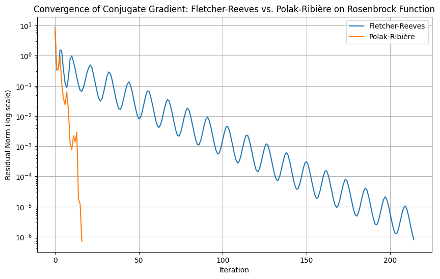
plt.title("Convergence of Conjugate Gradient: Fletcher-Reeves vs. Polak-Ribière on Rosenbrock Function")
plt.legend()
plt.grid(True)
plt.show()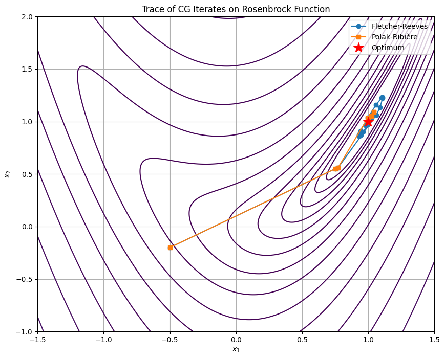

Summary¶

References¶

Nocedal, J., & Wright, S. J. (2006). Numerical optimization (Second Edition). Springer.

5.2 Nonlinear conjugate gradient methods

Motivation¶

Fletcher-Reeves vs Polyak-Ribière algorithms¶

Numerical illustration¶

Summary¶