5.1 Linear conjugate gradient method

In this section, we will consider the following square system of $n$ equations

where $x \in \mathbb{R}^n$, $Q \in \mathbb{R}^{n\times n}$ and $p\in \mathbb{R}^n$.

First, we recall that (1) is closely related to the study of least squares problems.

Preliminaries¶

Conjugacy property¶

Conjugate gradient methods rely on the conjugacy property.

Note that if $d_1, \ldots, d_\ell$ are conjugate with respect to $Q$, then they are linearly independent. (Prove it).

This property motivates a first algorithm, known as the conjugate direction method.

Conjugate directions method¶

Computation of the optimal stepsize $\alpha_k$

Let $\phi(\alpha) = \frac{1}{2} t(\alpha)^\top Qt(\alpha) - p^\top t(\alpha)$ where $t(\alpha) = x^{(k)}+\alpha d_k$. Hence $\alpha_k = \argmin_{\alpha} \phi(\alpha)$.

It is a quadratic convex function of $\alpha$, so it suffices to cancel out the derivative to get $\alpha_k$.

Define $r_k = Qx^{(k)}-p$ the residual at iteration $k$. Then

In addition, we have the following additional properties.

Proofs can be found in Nocedal & Wright (2006, p. 106), if interested.

The linear conjugate gradient (CG) method¶

The conjugate directions method of Algorithm 1 requires a set of conjugate directions $\lbrace d_k\rbrace$, which can be determined in advance using, e.g.,

• the eigenvalue decomposition of $Q$;

• a modification of the Gram-Schmidt process to produce a set of conjugate directions. This is, however, too costly for large scale applications.

Main idea and preliminary CG version¶

Choose the direction $d_k$ as a linear combination of $-r_k$ (negative residual) and $d_{k-1}$ (previous direction)

where $\beta_k$ is set to impose conjugation between $d_k$ and $d_{k-1}$:

This gives us a preliminary version of CG. Starting from $x^{(0)}\in \mathbb{R}^n$ and $d_0 = - r_0$, iterate until convergence

This first version is practical for studying properties of CG. To do this, we need to introduce the notion of Krylov subspace, which is very useful in numerical linear algebra..

Here are some important takeaways from the theorem:

• residuals $\lbrace r_k\rbrace$ are mutually orthogonal;

• Residuals $r_k$ and search directions $d_k$ all belong to the Krylov subspace of order $k$ associated with $r_0$;

• the search directions $d_0, d_1, \ldots, d_{N-1}$ are conjugate wrt $Q$

• by the conjugate direction theorem, this implies termination in at most $n$ steps.

• these results all depend on the choice of $d_0$! In fact, if one chooses $d_0 \neq - r_0$ (i.e., different from the steepest direction at $x^{(0)}$) then the theorem does not longer holds.

Practical CG algorithm¶

Using Property 1 and Theorem 2, we can improve the computations of $\alpha_k$ and $\beta_{k+1}$ in CG:

Moreover, observe that $r_{k+1}-r_k = \alpha_k Qd_k$ so that

where we used the orthogonality of residuals. This leads to the following practical algorithm.

Numerical illustration¶

Theorem 2 tells us convergence of CG to $x^\star$ is guaranteed after at most $n$ iterations. However, it can be much faster!

In fact,

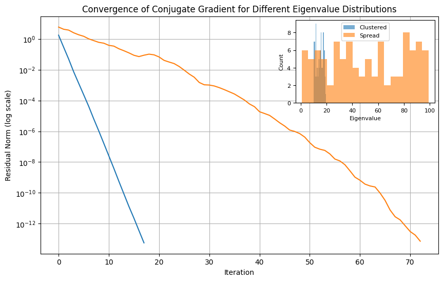
• convergence of CG usually depends on the \alert{distribution of eigenvalues of $Q$}

• it can be shown that if $Q$ has $r$ distinct eigenvalues, then CG converges in at most $r$ iterations.

The following example shows how CG convergence speed can be affected by the distrubution of eigenvalues.

import numpy as np
import matplotlib.pyplot as plt
from scipy.sparse.linalg import cg
from mpl_toolkits.axes_grid1.inset_locator import inset_axes

# Function to run CG on a system with matrix A and show convergence rates
def run_cg(A, b):
    x0 = np.zeros_like(b)
    residuals = []

    # Custom callback function to record residuals at each iteration
    def callback(xk):
        residuals.append(np.linalg.norm(b - A @ xk))

    # Run CG algorithm
    x, _ = cg(A, b, x0=x0, rtol=1e-14, callback=callback, maxiter=x0.size)
    return residuals

# Problem setup
n = 100
np.random.seed(10)
b = np.random.randn(n)

# Case 1: Well-clustered eigenvalues
eigenvalues_clustered = 10 + 10 * np.random.rand(n)
A_clustered = np.diag(eigenvalues_clustered)
residuals_clustered = run_cg(A_clustered, b)

# Case 2: Spread-out eigenvalues
eigenvalues_spread = 100 * np.random.rand(n)
A_spread = np.diag(eigenvalues_spread)
residuals_spread = run_cg(A_spread, b)

# Plot convergence rates
fig, ax = plt.subplots(figsize=(10, 6))
ax.semilogy(residuals_clustered, label="Clustered Eigenvalues")
ax.semilogy(residuals_spread, label="Spread Eigenvalues")
ax.set_xlabel("Iteration")
ax.set_ylabel("Residual Norm (log scale)")
ax.set_title("Convergence of Conjugate Gradient for Different Eigenvalue Distributions")
ax.grid(True)
ax.legend()

# Add inset for eigenvalue distributions
axins = inset_axes(ax, width="35%", height="35%", loc='upper right')
axins.hist(eigenvalues_clustered, bins=20, alpha=0.6, label="Clustered")
axins.hist(eigenvalues_spread, bins=20, alpha=0.6, label="Spread")
#axins.set_title("Eigenvalue Distribution", fontsize=10)
axins.set_xlabel("Eigenvalue", fontsize=8)
axins.set_ylabel("Count", fontsize=8)
axins.tick_params(axis='both', which='major', labelsize=8)
axins.legend(fontsize=8)

plt.show()

Summary¶