The mathematical toolbox - Mines Nancy

In this section we review some important concepts about objective functions $f:\mathbb{R}^n \to \mathbb{R}$ . We assume throughout that $f$ is (at least) continuously differentiable.

Convex functions¶

Recall from Chapter 2 two useful characterizations of convex functions.

Smooth functions¶

Another important notion is that of smoothness of a function $f$ , which relates to Lipschitz continuity properties of its gradient $\nabla f$ .

In particular, functions that are not differentiable, or differentiable with non-continuous derivatives are nonsmooth functions. Below are two important properties of smooth functions. On the other hand, if $f$ is $L$ -smooth, then this implies continuous differentiability of $f$ .

Proof

The proof is adapted from Wright & Recht (2022). Let $f$ be continuously differentiable. Recall the integral version of Taylor’s theorem

f(x + p) = f(x) + \int_0^1 \nabla f(x+ \gamma p )^\top p \mathrm{d}\gamma

(3)

for any $x, p \in \mathbb{R}^n$ . Then given $x, y \in \mathbb{R}^n$ we can build the quantity (using $x+p = y$ )

\begin{align*} f(y) - f(x) - \nabla f(x)^\top (y-x) = \int_0^1 \left[\nabla f(x + \gamma(y-x)) - \nabla f(x)\right]^\top (y-x)\mathrm{d}\gamma \end{align*}

(4)

Using $L$ -smoothness of $f$ , we bound the integrand as

\begin{align*} &\left[\nabla f(x + \gamma(y-x)) - \nabla f(x)\right]^\top (y-x)\\ & \leq \Vert \nabla f(x + \gamma(y-x)) - \nabla f(x) \Vert \cdot \Vert y -x\Vert & \text{(CS)}\\ & \leq L \gamma \Vert y - x \Vert^2 & \text{($L$-smoothness)} \end{align*}

(5)

Finally, by integrating the upper bound

\int_0^1 \left[\nabla f(x + \gamma(y-x)) - \nabla f(x)\right]^\top (y-x)\mathrm{d}\gamma \leq \frac{1}{2}L\Vert y - x \Vert^2

(6)

and thus the desired result

f(y) \leq f(x) + \nabla f(x)^\top (y-x) + \frac{1}{2}L\Vert y - x \Vert^2.

(7)

Noting $g_x: y \mapsto f(x) + \nabla f(x)^\top (y-x) + \frac{1}{2}L\Vert y - x \Vert^2$ we observe that $g_x(x) = f(x)$ ; $\nabla g_x(x) = \nabla f(x)$ ; $\nabla^2 g_x(x) = LI_n$ . This means that $f$ is upper bounded by a quadratic that takes, at $x$ , the same value $f(x)$ and gradient $\nabla f(x)$ , with Hessian $L I_n$ (curvature is $L$ in all directions).

Remark The notation $\nabla^2 f(x) \preceq L I_n$ means that the matrix $LI_n -\nabla^2 f(x)$ is positive semidefinite, or in other terms, the eigenvalues of the Hessian are upper-bounded by $L$ .

Proof

The proof is adapted from Wright & Recht (2022). We suppose that $f$ is twice continuously differentiable.

Suppose that $f$ is $L$ -smooth. Let $y = x + \alpha p$ and using Property 1, one gets
$f(x+\alpha p) - f(x) -\alpha \nabla f(x)^\top p \leq \frac{L}{2}\alpha^2 \Vert p \Vert^2.$
(8)
On the other hand, using Taylor’s theorem (second-order mean-value form) one gets
$f(x+\alpha p) - f(x) -\alpha \nabla f(x)^\top p = \frac{1}{2}\alpha^2 p^\top \nabla^2 f(x+\gamma \alpha p)p\quad \text{ for some }\gamma \in (0, 1)$
(9)
Comparing the two expressions we get the inequality
$p^\top \nabla^2 f(x+\gamma \alpha p)p \leq L \Vert p \Vert^2$
(10)
In the limit $\alpha \to 0$ , we get $p^\top \nabla^2 f(x)p \leq L \Vert p \Vert^2$ (using continuity of the Hessian). Taking $p$ as any of eigenvectors of $\nabla^2 f(x)$ shows that the associated eigenvalues is bounded by $L$ . Hence, $\nabla^2 f(x) \preceq L I_n$ .
Suppose that $-LI_n \preceq \nabla^2 f(x) \preceq LI_n$ for all $x$ . As a result, the operator norm $\Vert\nabla^2 f(x)\Vert_2 = \max(\vert \lambda_1\vert, \ldots, \vert \lambda_n\vert)$ where the $\lambda_i$ are the eigenvalues of $\nabla^2 f(x)$ . Since by assumptions all eigenvalues are smaller than $L$ (in absolute value), we get $\Vert \nabla^2 f(x)\Vert_2 \leq L$ . Now, recall another version of Taylor’s theorem, i.e.,
$\nabla f(x+p) = \nabla f(x) + \int_0^1 \nabla^2 (x+\gamma p)p \mathrm{d}\gamma$
(11)
We can apply directly this result to bound $\Vert \nabla f(y)-\nabla f(x)\Vert$ as
$\begin{align*} \Vert \nabla f(y)-\nabla f(x)\Vert &= \left\Vert \int_0^1 \nabla^2 (x+\gamma (y-x))(y-x) \mathrm{d}\gamma \right\Vert & \text{(Taylor's theorem)}\\ & \leq \int_0^1 \left\Vert \nabla^2 (x+\gamma (y-x))\right\Vert\Vert y-x \Vert \mathrm{d}\gamma &\\ &\leq \int_0^1 L \Vert y -x \Vert \mathrm{d}\gamma& \text{(bounded operator norm)}\\ & = L\Vert y -x \Vert& \end{align*}$
(12)
which shows that $f$ is $L$ -smooth.

Strong convexity¶

Remarks

the definition can be extended to non-differentiable functions
if $f$ is $m$ -strongly convex, then $f$ is also strictly convex
the function $f$ is $m$ -strongly convex iff $g(x) = f(x) - \frac{m}{2}\Vert x \Vert_2^2$ is convex

The following properties are direct consequences of strong convexity and / or smoothness applied to convex functions.

This result shows that Hessian eigenvalues are lower-bounded by $m$ .

Proof

$\Rightarrow$ . Suppose that $f$ is $m$ -strongly convex. For any $x, p \in \mathbb{R}^N$ and $\alpha > 0$ , Taylor’s theorem gives
$f(x+\alpha p) = f(x) + \alpha \nabla f(x)^\top p + \frac{1}{2}\alpha^2 p^\top \nabla^2 f(x+\gamma \alpha p) p \text{ for some }\gamma \in (0, 1).$
(14)
Using the strong convexity property, one gets
$f(x+\alpha p) \geq f(x) + \alpha \nabla f(x)^\top p + \frac{m}{2}\alpha^2\Vert p\Vert^2$
(15)
Plugging the two statements into one another, one gets the inequality
$p^\top \nabla^2 f(x+\gamma \alpha p) p \geq m \Vert p\Vert^2$
(16)
As before, taking the limit $\alpha \rightarrow 0$ , one has $p^\top \nabla^2 f(x) p \geq m \Vert p\Vert^2$ and thus $\nabla^2 f(x) \succeq m I_n$ .
$\Leftarrow$ . Suppose that $\nabla^2 f(x) \succeq m I_n$ . Using once again Taylor’s theorem,
$f(y) = f(x) + \nabla f(x)^\top (y-x) + \frac{1}{2}(y-x)^\top \nabla^2 f(x + \gamma (y-x)) (y-x)\text{ for some }\gamma \in (0, 1).$
(17)
Since $\nabla^2 f(x) \succeq m I_n$ this means that $\nabla^2 f(x)- m I_n\succeq 0$ , hence for any $z, x\in \mathbb{R}^N$ one has $z^\top (\nabla^2 f(x)- m I_n)z \geq 0$ , i.e., $z^\top \nabla^2 f(x)z \geq m \Vert z\Vert^2$ . Thus,
$(y-x)^\top \nabla^2 f(x + \gamma (y-x)) (y-x) \geq m \Vert y -x \Vert^2$
(18)
and
$f(y) \geq f(x) + \nabla f(x)^\top (y-x) + \frac{1}{2}m \Vert y -x\Vert^2$
(19)
which shows that $f$ is $m$ -strongly convex.

Another property is the following.

Proof

Let $f$ be a twice differentiable convex function.

$\Rightarrow$ suppose that $f$ is $L$ -smooth. Then by Property 2, $\nabla^2 f(x) \preceq L I_n$ . Moreover, since $f$ is convex, $\nabla^2 f(x)\succeq 0$ , so that $0\preceq \nabla^2 f(x)\preceq L I_n$ .
$\Leftarrow$ Suppose that $0\preceq \nabla^2 f(x)\preceq L I_n$ . Then, in particular $-LI_n\preceq \nabla^2 f(x)\preceq L I_n$ . By Property 2, $f$ is $L$ -smooth.

Summary: smoothness and strong convexity¶

The following numerical example illustrates how for a given function $f$ , its properties (convexity, smoothness, strong convexity) permit to “bound” the function on its domain by simple (linear or quadratic) functions.

Let us consider $f: x \mapsto \frac{1}{2}x^2$ . The function is obviously convex, $L$ -smooth (for any $L \geq 1$ ) and $m$ -strongly convex (for any $0< m \leq 1$ ). Then we can display the upper and lower bounds induced by considering the smoothness, convexity and strong convexity alone - or by combining them. These bounds become ultimately important when one wants to characterize convergence properties of optimization algorithms.

import numpy as np
import matplotlib.pyplot as plt
import palettable as pal
from ipywidgets import interact, FloatSlider

cmap = pal.colorbrewer.qualitative.Paired_4.mpl_colors

myblue = cmap[1]
mygreen = cmap[3]
def f(x):
    return 0.5*x**2

def gradf(x):
    return x

def upper_bound(x0, x, L):
    y = f(x0) + gradf(x0)*(x-x0) + 0.5*L*(x-x0)**2
    return y

def lower_bound(x0, x, m):
    y = f(x0) + gradf(x0)*(x-x0) + 0.5*m*(x-x0)**2
    return y

x = np.linspace(-1,2, 100)
L = 1.5
m = 0.6

def plot_bounds(x0):
    fig, ax = plt.subplots(figsize=(12, 8), ncols=2, nrows=2, sharex=True, sharey=True)

    # L-smoothness
    ax[0, 0].plot(x, f(x), color=myblue, linewidth=2)
    ax[0, 0].plot(x, upper_bound(x0, x, L), color=mygreen, linewidth=2)
    ax[0, 0].plot(x, upper_bound(x0, x, -L), color=mygreen, linewidth=2)
    ax[0, 0].fill_between(x, upper_bound(x0, x, -L),\
        upper_bound(x0, x, L), alpha=0.1, color=mygreen)
    ax[0, 0].scatter(x0, f(x0), marker='o', color='k', zorder=10)

    # strong convexity
    ax[0, 1].plot(x, f(x), color=myblue, linewidth=2)
    ax[0, 1].plot(x, lower_bound(x0, x, m), color=mygreen, linewidth=2)
    ax[0, 1].fill_between(x, lower_bound(x0, x, m), 2, alpha=0.1, color=mygreen)
    ax[0, 1].scatter(x0, f(x0), marker='o', color='k', zorder=10)

    # L-smooth, convex
    ax[1, 0].plot(x, f(x), color=myblue, linewidth=2)
    ax[1, 0].plot(x, upper_bound(x0, x, L), color=mygreen, linewidth=2)
    ax[1, 0].plot(x, upper_bound(x0, x, 0), color=mygreen, linewidth=2)
    ax[1, 0].fill_between(x, upper_bound(x0, x, 0),\
        upper_bound(x0, x, L), alpha=0.1, color=mygreen)
    ax[1, 0].scatter(x0, f(x0), marker='o', color='k', zorder=10)

    # L-smooth, m-strg convex
    ax[1, 1].plot(x, f(x), color=myblue, linewidth=2)
    ax[1, 1].plot(x, upper_bound(x0, x, L), color=mygreen, linewidth=2)
    ax[1, 1].plot(x, lower_bound(x0, x, m), color=mygreen, linewidth=2)
    ax[1, 1].fill_between(x, lower_bound(x0, x, m),\
        upper_bound(x0, x, L), alpha=0.1, color=mygreen)
    ax[1, 1].scatter(x0, f(x0), marker='o', color='k', zorder=10)

    # clean
    for axis in np.ravel(ax):
        axis.xaxis.set_visible(False)
        axis.yaxis.set_visible(False)
        for side in ['top','right','bottom','left']:
            axis.spines[side].set_visible(False)

    fig.tight_layout()
    ax[0, 0].set_ylim(-.2, 1)
    labelsize=20
    ax[0, 0].set_title('$L$-smooth', size=labelsize, y=0.9)
    ax[0, 1].set_title('$m$-strongly convex', size=labelsize, y=0.9)
    ax[1, 0].set_title('$L$-smooth, convex', size=labelsize, y=0.9)
    ax[1, 1].set_title('$L$-smooth, $m$-strongly convex', size=labelsize, y=0.9)
    plt.show()

interact(plot_bounds, x0=FloatSlider(value=0.5, min=-1, max=2, step=0.01, description='$x_0$'));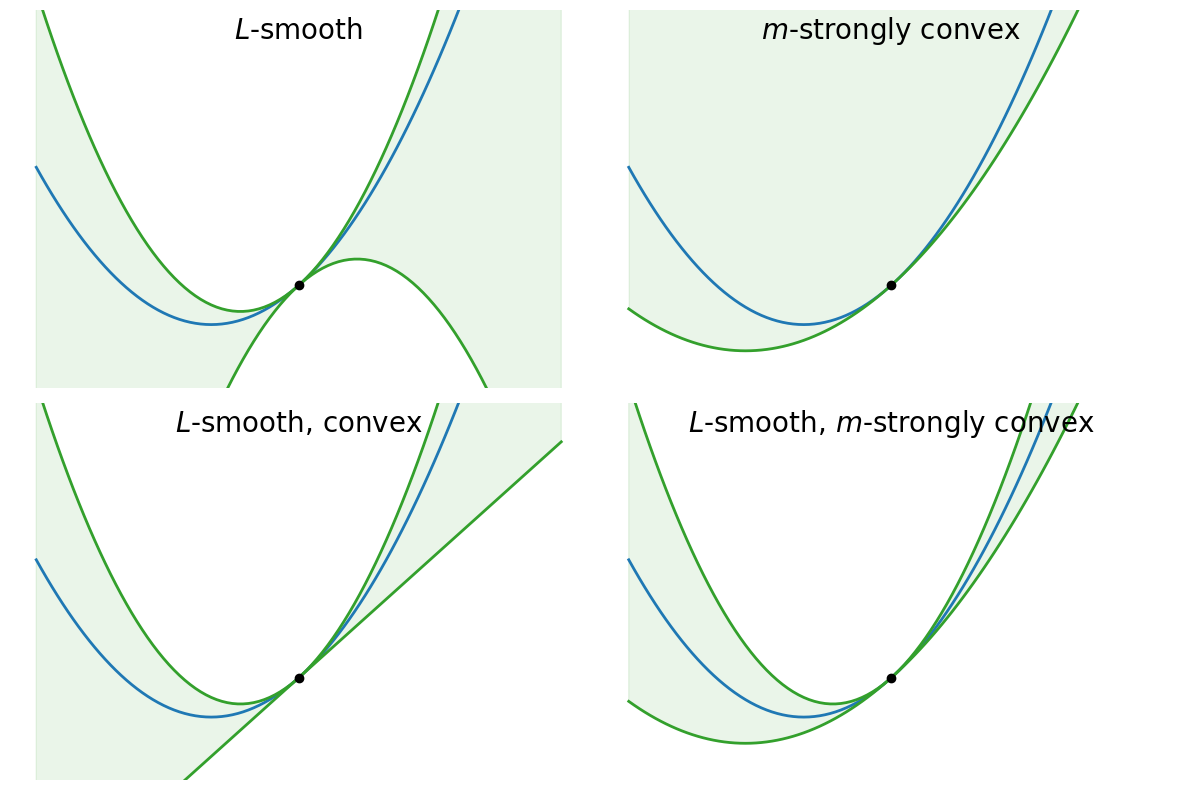

Assessing convergence¶

The kind of convergence guarantees strongly depend on the regularity properties (convexity, smoothness, strong convexity) of the objective $f$ :

Convergence in objective function values: In this case, we bound the distance to the optimal value $f( x^{(k)}) - f(x^\star)$ . This condition is usually weaker and requires less assumptions about $f$ .
Convergence in iterates: Here, we bound the distance between the current iterate and a optimal point $x^\star$ , $\Vert x^{(k)} - x^\star\Vert_2$ . This usually requires strong convexity of $f$ .

In some cases, both type of convergence can be related.

References¶

Wright, S. J., & Recht, B. (2022). Optimization for data analysis. Cambridge University Press.

6.1 The mathematical toolbox

Convex functions¶

Smooth functions¶

Strong convexity¶

Summary: smoothness and strong convexity¶

Assessing convergence¶