Quasi-Newton methods - Mines Nancy

Motivation¶

Despite its numerous advantages, Newton’s method suffers from two disadvantages:

Computing Newton’s step involves calculating and inverting the Hessian matrix $\nabla^2 f_0(x^{(k)})$ , which becomes very costly in high dimensions.
The Hessian matrix $\nabla^2 f_0(x^{(k)})$ is not always positive definite, so it’s not always possible to calculate its inverse.

Solution: We replace the Hessian matrix with an approximation $B_k \approx \nabla^2 f_0(x^{(k)})$ , leading to so-called quasi-Newton methods.

Principle of Quasi-Newton Methods¶

The crucial step lies in defining matrices $B_k$ (or $H_k$ ) such that

B_k \approx \nabla^2 f_0(x^{(k)}) \quad \text{or} \quad H_k \approx \left[\nabla^2 f_0(x^{(k)})\right]^{-1}

(2)

often by a recursive relation (i.e., it is built on the fly, from values at previous iterations). For a given update rule, one gets a specific quasi-Newton method. Some examples are:

Broyden-Fletcher-Goldfarb-Shanno (BFGS), probably the most popular
L-BFGS: memory-efficient BFGS
Symmetric rank-one (SR1)
Davidon–Fletcher–Powell (DFP), etc.

Many of such algorithms are implemented in standard Python libraries, such as in scipy. Check for instance the documentation of scipy.optimize.minimize function.

Example: BFGS algorithm¶

Algorithm 2 (BFGS)

Given initial point $x^{(0)}$ and initial $H_0$ , at the $k$ -th iteration, do

$x^{(k+1)} = x^{(k)} - \alpha_k H_k \nabla f_0(x^{(k)})$
$s_k = -\alpha_k H_k \nabla f_0(x^{(k)}), \quad y_k = \nabla f_0(x^{(k+1)}) - \nabla f_0(x^{(k)}), \quad \rho_k = \frac{1}{s_k^\top y_k}$
$H_{k+1} = \left(I_n - \rho_k s_ky_k^\top\right)H_k\left(I_n - \rho_k y_ks_k^\top\right) + \rho_k s_ks_k^\top$

and repeat steps 1-2-3 until convergence.

For details about the derivation of BFGS updates, properties of the algorithm and implementation details, one can consult Section 6.1, Nocedal & Wright, 2006.

Comparison on a non-quadratic example¶

To compare the BFGS algorithm with gradient descent (fixed step-size) and Newton’s method, we come back to the non-quadratic example introduced when studying step-size strategies for gradient descent

\begin{array}{ll} \minimize &\quad f_0(x):=e^{x_1+3x_2 - 0.1} + e^{x_1 -3x_2 - 0.1} + e^{-x_1 - 0.1}\\ \st & \quad x \in \mathbb{R}^2 \end{array}

(3)

Let us look at how fixed step-size gradient descent and Newton’s method perform on this problem.

import numpy as np
import matplotlib.pyplot as plt
from scipy.optimize import minimize

def f(x1, x2):
    return np.exp(x1 +3*x2 - 0.1) + np.exp(x1 -3*x2- 0.1) + np.exp(-x1 - 0.1)

def dfdx(x1, x2):
    dx1 = np.exp(x1 + 3*x2 - 0.1) + np.exp(x1 - 3*x2 - 0.1) - np.exp(-x1 - 0.1)
    dx2 = 3 * np.exp(x1 + 3*x2 - 0.1) - 3 * np.exp(x1 - 3*x2 - 0.1)
    return np.array([dx1, dx2])

def d2fd2x(x1, x2):
    hess = np.array([
        [
            np.exp(x1 + 3*x2 - 0.1) + np.exp(x1 - 3*x2 - 0.1) + np.exp(-x1 - 0.1),
            3*np.exp(x1 + 3*x2 - 0.1) - 3*np.exp(x1 - 3*x2 - 0.1)
        ],
        [
            3*np.exp(x1 + 3*x2 - 0.1) - 3*np.exp(x1 - 3*x2 - 0.1),
            9*np.exp(x1 + 3*x2 - 0.1) + 9*np.exp(x1 - 3*x2 - 0.1)
        ]
    ])
    return hess

def gradient_descent(xinit, dfdx, alpha, niter=10):
    xn = np.zeros((2, niter + 1))
    xn[:, 0] = xinit
    for n in range(niter):
        grad = dfdx(xn[0, n], xn[1, n])
        xn[:, n + 1] = xn[:, n] - alpha * grad
    return xn

def newton_method(xinit, dfdx, d2fd2x, niter=10):
    xn = np.zeros((2, niter + 1))
    xn[:, 0] = xinit
    for n in range(niter):
        grad = dfdx(xn[0, n], xn[1, n])
        hess = d2fd2x(xn[0, n], xn[1, n])
        xn[:, n + 1] = xn[:, n] - np.linalg.pinv(hess) @ grad
    return xn
def plot_path(xs, label):
    xs = np.array(xs)
    plt.plot(xs[0,:], xs[1,:], marker='o', label=label)


# starting point
xinit = [-2, .5]
alpha = 0.1
xn_grad = gradient_descent(xinit, dfdx, alpha, niter=50)
xn_newton = newton_method(xinit, dfdx, d2fd2x, niter=20)

# plot
x1s = np.linspace(-2, 0.6, 50)
x2s = np.linspace(-0.5, 0.5, 50)
X1, X2 = np.meshgrid(x1s, x2s)
Z = f(X1, X2)

plt.figure(figsize=(8, 6))
cp = plt.contourf(X1, X2, Z, levels=30, cmap='viridis')
plot_path(xn_grad, r"Fixed step-size $\alpha$" + f"$= {alpha}$")
plot_path(xn_newton, "Newton's method")
plt.legend()

plt.colorbar(cp)
plt.xlabel("$x_1$")
plt.ylabel("$x_2$")
plt.title("$f_0$")
plt.show()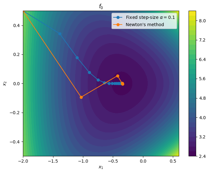

Below is a possible, non-optimized, BFGS implementation.

def BFGS(xinit, dfdx, Hinit, alphainit, f, niter=10, s=0.3, eta=0.9):
    xn = np.zeros((2, niter + 1))
    xn[:, 0] = xinit
    Hk = Hinit
    grad = dfdx(xn[0, 0], xn[1, 0])
    for n in range(niter):
        alpha = alphainit
        xtemp = xn[:, n] - alpha * Hk @ grad

        # check backtracking condition
        ftemp = f(xtemp[0], xtemp[1])
        backtrack_comp = f(xn[0, n], xn[1, n]) - alpha * s * grad.T @ Hk @ grad
        while ftemp > backtrack_comp:
            alpha = eta * alpha
            xtemp = xn[:, n] - alpha * Hk @ grad
            ftemp = f(xtemp[0], xtemp[1])
            backtrack_comp = f(xn[0, n], xn[1, n]) - alpha * s * grad.T @ Hk @ grad

        xn[:, n + 1] = xtemp

        # update Hk
        if n < niter - 1:
            newgrad = dfdx(xn[0, n + 1], xn[1, n + 1])
            sk = xn[:, n + 1] - xn[:, n]
            yk = newgrad - grad
            rhok = 1.0 / (yk.T @ sk)
            grad = newgrad
            I = np.eye(2)
            mat = I - rhok * np.outer(sk, yk)
            mat2 = I - rhok * np.outer(yk, sk)
            Hk = mat @ Hk @ mat2 + rhok * np.outer(sk, sk)
    return xn

Let us compare how BFGS performs, starting from the same initial point and using $H_0 = [\nabla^2 f(x^{(0)})]^{-1}$ .

# BFGS
Hinit = np.linalg.pinv(d2fd2x(xinit[0], xinit[1]))
xn_BFGS = BFGS(xinit, dfdx, Hinit, 1, f, niter=10, s=0.3, eta=0.5)
# plot
x1s = np.linspace(-2, 0.6, 50)
x2s = np.linspace(-0.5, 0.5, 50)
X1, X2 = np.meshgrid(x1s, x2s)
Z = f(X1, X2)

plt.figure(figsize=(8, 6))
cp = plt.contourf(X1, X2, Z, levels=30, cmap='viridis')
plot_path(xn_grad, r"GD with fixed step-size $\alpha$" + f"$= {alpha}$")
plot_path(xn_newton, "Newton's method")
plot_path(xn_BFGS, "BFGS")
plt.legend()

plt.colorbar(cp)
plt.xlabel("$x_1$")
plt.ylabel("$x_2$")
plt.title("$f_0$")
plt.show()

# compute optimal value
res = minimize(lambda x: f(x[0], x[1]), xinit)
pstar = res.fun

# Plot objective values for each method
plt.figure(figsize=(8, 6))
plt.semilogy([f(*x) - pstar for x in xn_grad.T], label=r"GD with fixed step-size $\alpha$" + f"$= {alpha}$", marker='o')
plt.semilogy([f(*x)- pstar for x in xn_newton.T], label="Newton's method", marker='o')
plt.semilogy([f(*x)- pstar for x in xn_BFGS.T], label=f"BFGS", marker='o')
plt.xlabel("Iteration")
plt.ylabel("$f_0(x) - p^\star$")
plt.title("suboptimality value vs iteration")
plt.legend()
plt.grid(True)
plt.show()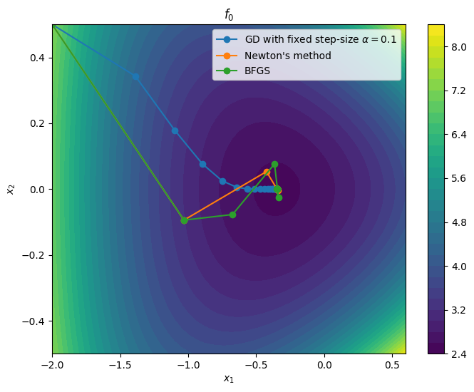

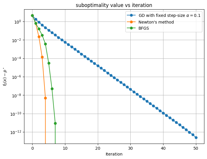
In this example, we see that BFGS does converges almost as fast as Newton’s method -- and much faster than fixed step-size gradient descent. However, unlike Newton’s method, it does not require the evaluation of the Hessian at each iteration.

References¶

Nocedal, J., & Wright, S. J. (2006). Numerical optimization (Second Edition). Springer.

Mines Nancy - Optimization course

Newton’s method

Mines Nancy - Optimization course

Algorithms for nonlinear least-squares problems

4.5Quasi-Newton methods

Motivation¶

Principle of Quasi-Newton Methods¶

Example: BFGS algorithm¶

Comparison on a non-quadratic example¶