4.4Newton’s method

We deal with the unconstrained optimization problem

We assume that $f_0$ is twice continuously differentiable. The Newton’s method (or Newton’s algorithm) attempts at solving (1) using the following strategy.

Newton’s method requires the function to have positive definite Hessian at iterates $x^{(k)}$: indeed it requires to compute $\left[\nabla^2 f_0(x^{(k)})\right]^{-1}$, which is only defined when the Hessian is invertible (or equivalently, positive definite since it is symmetric). When it is the case, the direction $d_k = -\left[\nabla^2 f_0(x^{(k)})\right]^{-1}\nabla f_0(x^{(k)})$ is indeed a descent direction since

invoking positive definiteness of the Hessian at $x^{(k)}$.

Example for quadratic functions¶

Consider the quadratic function

where $Q \in \mathbb{R}^{n \times n}$ is symmetric positive definite, $p \in \mathbb{R}^n$, and $c \in \mathbb{R}$. The gradient and Hessian are:

Note that since $Q \succ 0$ by assumption, $f_0$ is strictly convex and has a unique minimizer given by $x^\star = Q^{-1} p$.

Applying Newton’s method with constant step size $\alpha_k = 1$

Newton’s method finds the minimizer in a single iteration, regardless of the starting point $x^{(0)}$! On the other hand, if $\alpha_k = \alpha \in (0, 1)$, one has

Hence, by recurrence, we get

which converges to $x^\star$ as $k\to \infty$.

Newton step as minimizer of the local quadratic approximation¶

Newton’s method can be motivated by considering a local quadratic approximation of the objective function $f_0$. Around a point $x^{(k)}$, the second-order Taylor expansion of $f$ is

where the linear term captures first-order behavior and the quadratic term incorporates curvature information through the Hessian $\nabla^2 f_0(x^{(k)})$.

Let $p = x - x^{(k)}$ denote the step direction. Define the local quadratic model:

which is a quadratic function of $p$. Assuming the Hessian is positive definite, this function is strictly quadratic and thus the (unique) minimizer of $m_k(p)$ satisfies the first-order optimality condition

Solving for $p$ gives

Thus, the update rule is

which is exactly the Newton step of Algorithm 1 above, for $\alpha_k = \alpha=1$.

Implications and discussion¶

The fact that the Newton step can be interpreted as the minimization of the local quadratic approximation has several important implications:

• whenever $x^{(k)}$ is sufficiently close to a local optimum $x^\star$, higher-order terms become negligible, so Newton’s method exhibits quadratic convergence. This explains why Newton’s method can rapidly “lock in” on the solution once it is sufficiently close.
• however, far from the local optimum, the local quadratic approximation might not be very accurate: in this setting, the algorithm may even diverge. In practice, we implement backtracking to ensure sufficient decrease of the objective through the choice of the stepsize $\alpha_k$.
• Newton’s methods leverages the second-order information stored in the Hessian. This allows the algorithm to adapt to the local curvature of the objective function and potentially escape slow progress in ill-conditioned regions.

There are two important shortcomings to keep in mind:

• Computing and inverting the Hessian matrix at each iteration can be computationally expensive, especially for large-scale problems.
• The method requires the Hessian to be positive definite and invertible at each step; otherwise, the direction may not be a descent direction or may not be defined at all.

These issues are addressed (in part) by quasi-Newton methods, as discussed in the next section.

Example¶

We consider the minimization problem of the Rosenbrock function in 2D.

which has a clear (global) optima at $x^\star = [1, 1]^\top$ with optimal value $p^\star = 0$.

Source

import numpy as np
import matplotlib.pyplot as plt

# Rosenbrock function
def f(v):
    x, y = v
    return (1 - x)**2 + 100*(y - x**2)**2

def grad(v):
    x, y = v
    return np.array([
        -2*(1-x) - 400*x*(y - x**2),
        200*(y - x**2)
    ])

def hess(v):
    x, y = v
    return np.array([
        [2 - 400*y + 1200*x**2, -400*x],
        [-400*x, 200]
    ])

# Gradient Descent
def gradient_descent(x0, alpha=0.002, max_iter=5000):
    x = x0.copy()
    xs = [x.copy()]
    for _ in range(max_iter):
        x -= alpha * grad(x)
        xs.append(x.copy())
        if np.linalg.norm(grad(x)) < 1e-6:
            break
    return np.array(xs)

# Newton's Method with damping (line search)
def newton_method(x0, max_iter=50):
    x = x0.copy()
    xs = [x.copy()]
    for _ in range(max_iter):
        g = grad(x)
        H = hess(x)

        p = np.linalg.pinv(H) @ g
        x -=  p
        xs.append(x.copy())
    return np.array(xs)

# Run both methods
x0 = np.array([-0.5, 0.1])  # common starting point
gd_path = gradient_descent(x0)
newton_path = newton_method(x0)

# Contour plot
xx, yy = np.meshgrid(np.linspace(-1.5, 1.5, 400), np.linspace(-1, 2, 400))
zz = (1-xx)**2 + 100*(yy-xx**2)**2

plt.figure(figsize=(8,6))
plt.contourf(xx, yy, zz, levels=40, cmap="viridis")

plt.plot(gd_path[:,0], gd_path[:,1], 'o--', label="Gradient Descent ($\\alpha=0.002$)")
plt.plot(newton_path[:,0], newton_path[:,1], 's--', label="Newton's Method ($\\alpha=1$)")

plt.plot(1, 1, 'r*', markersize=12, label="Minimum")
plt.colorbar()
plt.title("Newton vs Gradient Descent on the Rosenbrock Function")
plt.xlabel("x")
plt.ylabel("y")
plt.legend()
plt.show()

# Plot convergence in objective values
plt.figure(figsize=(8, 4))
plt.semilogy([f(x) for x in gd_path], label="Gradient Descent ($\\alpha=0.002$)")
plt.semilogy([f(x) for x in newton_path], label="Newton's Method ($\\alpha=1$)")
plt.xlabel("Iteration")
plt.ylabel("Objective value $f(x)$")
plt.title("Convergence of objective values")
plt.legend()
plt.grid(True)
plt.show()

# Zoom on the first 20 iterations
plt.figure(figsize=(8, 4))
plt.semilogy(range(20), [f(x) for x in gd_path[:20]], 'o-', label="Gradient Descent (first 20)")
plt.semilogy(range(20), [f(x) for x in newton_path[:20]], 's-', label="Newton's Method (first 20)")
plt.xlabel("Iteration")
plt.ylabel("Objective value $f(x)$")
plt.title("Zoom: First 20 Iterations")
plt.legend()
plt.grid(True)
plt.show()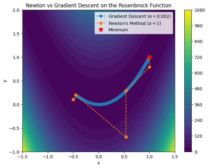

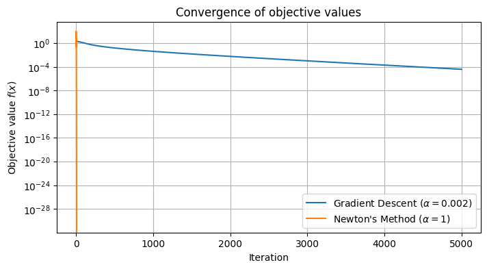
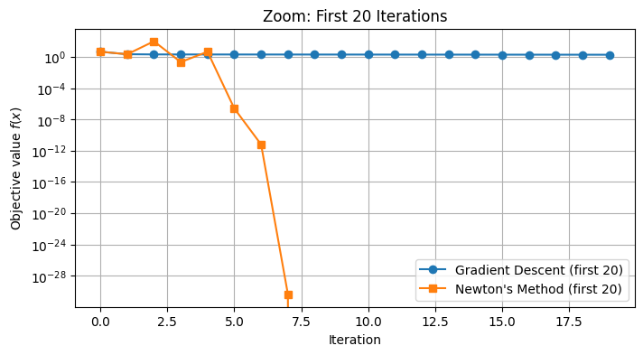
On this example, the difference between gradient descent and Newton’s method is illuminating. While gradient descent requires many small steps to navigate the curved valley of the Rosenbrock function, Newton’s method quickly adjusts its trajectory and reaches the optimum in far fewer iterations, thanks to its use of second-order information. This illustrates the practical advantage of Newton’s method when the Hessian is available and well defined.