2.4 Optimality conditions for unconstrained optimization
First, we consider the unconstrained optimization problem
minimize f 0 ( x ) subject to x ∈ R n \begin{array}{ll}
\minimize& f_0({x})\\
\st & x \in \mathbb{R}^n
\end{array} minimize subject to f 0 ( x ) x ∈ R n We assume that f 0 f_0 f 0 R n \mathbb{R}^n R n f 0 f_0 f 0
Provided optima exist (not always guaranteed!), we will derive conditions on a point x ⋆ x^\star x ⋆ local optimum of the problem. (in the unconstrained case, one also says that x ⋆ x^\star x ⋆ local minimizer of f 0 f_0 f 0 global optimality , we’ll need to assume convexity of the objective function f 0 f_0 f 0
Most of the results from this section are reproduced from Nocedal & Wright (2006, Chapter 2)
Necessary conditions (unconstrained case) ¶ We call x ⋆ x^\star x ⋆ stationary or critical point of f 0 f_0 f 0 ∇ f 0 ( x ⋆ ) = 0 \nabla f_0(x^\star) = 0 ∇ f 0 ( x ⋆ ) = 0
Any local optima must be a stationary point.
Prove Theorem 1 Theorem 2
Theorem 1 Theorem 2 necessary conditions for a point x ⋆ x^\star x ⋆
For higher dimensions (here 2D), the situation is even more subtle.
Sufficient conditions (unconstrained case) ¶ Suppose that ∇ 2 f 0 \nabla^2 f_0 ∇ 2 f 0 x ⋆ x^\star x ⋆ ∇ f 0 ( x ⋆ ) = 0 \nabla f_0(x^\star) = 0 ∇ f 0 ( x ⋆ ) = 0 ∇ 2 f 0 ( x ⋆ ) ≻ 0 \nabla^2 f_0(x^\star) \succ 0 ∇ 2 f 0 ( x ⋆ ) ≻ 0 x ⋆ x^\star x ⋆ (1) x ⋆ x^\star x ⋆ f 0 f_0 f 0
Sufficient conditions guarantee that local optima are strict , i.e. they are isolated. (Compare with the necessary conditions of Theorem 1 Theorem 2
These sufficient conditions are not necessary: a point x ⋆ x^\star x ⋆ f 0 f_0 f 0
Example: f ( x ) = x 4 f(x) = x^4 f ( x ) = x 4 x ⋆ = 0 x^\star = 0 x ⋆ = 0 f ′ ′ ( 0 ) = 0 f''(0) = 0 f ′′ ( 0 ) = 0
Exercise 2 (Quadratic function)
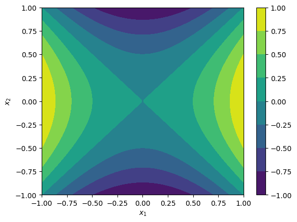
Let f : R 2 → R f:\mathbb{R}^2 \rightarrow \mathbb{R} f : R 2 → R f ( x ) = x 1 2 − x 2 2 f(x) = x_1^2 - x_2^2 f ( x ) = x 1 2 − x 2 2
To help, here is how to plot this function in Python.
import numpy as np
import matplotlib.pyplot as plt

u = np.linspace(-1, 1, 128)
x1, x2= np.meshgrid(u, u)

plt.contourf(x1, x2, x1**2-x2**2)
plt.colorbar()
plt.xlabel(r'$x_1$')
plt.ylabel(r'$x_2$');
Exercise 3 (Rosenbrock function)
Let f : R 2 → R f:\mathbb{R}^2 \rightarrow \mathbb{R} f : R 2 → R f ( x ) = ( 1 − x 1 ) 2 + 5 ( x 2 − x 1 2 ) 2 f(x) = (1-x_1)^2 + 5(x_2-x_1^2)^2 f ( x ) = ( 1 − x 1 ) 2 + 5 ( x 2 − x 1 2 ) 2
Does the point [ 1 , 1 ] ⊤ [1, 1]^\top [ 1 , 1 ] ⊤
Necessary and sufficient conditions (unconstrained case) ¶ When f 0 f_0 f 0
Consider the unconstrained optimization problem (1) f 0 : R n → R f_0:\mathbb{R}^n\rightarrow \mathbb{R} f 0 : R n → R x ⋆ x^\star x ⋆ Theorem 3 x ⋆ x^\star x ⋆ f 0 f_0 f 0 ∇ f 0 ( x ⋆ ) = 0 \nabla f_0(x^\star) = 0 ∇ f 0 ( x ⋆ ) = 0
If f 0 f_0 f 0
Finding points such that ∇ f 0 ( x ⋆ ) = 0 \nabla f_0 (x^\star) = 0 ∇ f 0 ( x ⋆ ) = 0
In chapter 3, we’ll see a very important application of this result to solve a very important category of optimization problems, called (unconstrained) least-squares problems.
Nocedal, J., & Wright, S. J. (2006). Numerical optimization (Second Edition). Springer.