3.2General form of (linear) least squares problems

The main hypothesis is that there exists a linear relationship between data $y \in \mathbb{R}^m$ and variables $x \in \mathbb{R}^n$.

Definitions and Notations¶

• The vector $y \in \mathbb{R}^m$ contains the data, also named observations or measurements, which we want to model;
• The matrix $A \in \mathbb{R}^{m\times n}$ encodes the model (assumed known).
• The vector $x\in \mathbb{R}^n$ represents the unknowns.
• The vector $b \in \mathbb{R}^m$ expresses errors (model, noise, etc.).

For simplicity, we assume that observations $y_1, \ldots y_n$ are linearly independent. This is equivalent to saying that observations are not redundant. The problem (1) is said to be

• overdetermined when $m \geq n$ (more observations than unknowns)
• underdetermined when $m \leq n$ (strictly less observations than unknowns)

The over/under determination property play an important role regarding the uniqueness of solutions to the least squares problem, as we will see later on.

Interpretation as an unconstrained quadratic program (QP)¶

The objective function $f_0(x) = \Vert y - Ax\Vert_2^2$ can be rewritten as

such that the least-squares optimization problem can be equivalently reformulated as the unconstrained quadratic program

where $Q:= A^\top A \in \mathbb{R}^{n\times n}$ and $p := A^\top y \in \mathbb{R}^n$.

Examples¶

Polynomial regression¶

Assume we are given some data $y_1, \ldots, y_m$ as a function of time $t$, as shown below:

Source

import numpy as np
import matplotlib.pyplot as plt

np.random.seed(2025)
def f(x):
    return x**3 + 4*x**2 - x + 1

N = 20
ts = np.linspace(-4., 2., N)

y = f(ts) + np.random.randn(N)
plt.scatter(ts, y, label="data $y$")
plt.xlabel(r"$t$")
plt.ylabel(r"$y$")
plt.legend()
plt.show()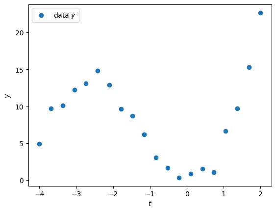

The trend clearly looks polynomial. If we assume the degree $d$ of the polynomial is known (here $d=3$), we can write a linear model to fit the data $y$. The approach very classical: hence it is implemented in many libraries, such as scikit-learn (see PolynomialFeatures and LinearRegression).

from sklearn.preprocessing import PolynomialFeatures
from sklearn.linear_model import LinearRegression

# construct polynomial regression matrix
degree = 3
poly = PolynomialFeatures(degree)
X_poly = poly.fit_transform(ts.reshape(-1, 1))

# fit the data (solve the LS problem)
model = LinearRegression(fit_intercept=False)
model.fit(X_poly, y)
y_pred = model.predict(X_poly)

# display results
plt.scatter(ts, y, label="data $y$")
plt.plot(ts, f(ts), color="green", linestyle="--", label="ground truth")
plt.plot(ts, y_pred, color="red", label=f"degree {degree} fit")
plt.xlabel("$t$")
plt.ylabel("$y$")
plt.legend()
plt.show()

# Print the estimated polynomial coefficients
print("Estimated coefficients (in increasing powers of t):\n", model.coef_)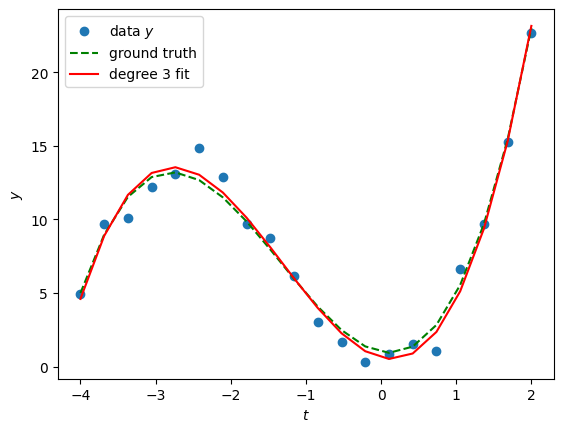

Estimated coefficients (in increasing powers of t):
 [ 0.61187122 -1.2593056   4.15376347  1.05475994]

In TP1, we will see what’s under the hood of such tools and implement the solution from scratch.

2D image deconvolution¶

Assume we observe a blurred image $Y \in \mathbb{R}^{H \times W}$, which is the result of convolving a true image $X \in \mathbb{R}^{n_H \times n_W}$ with a known kernel $K \in \mathbb{R}^{k_H \times k_W}$, plus noise $B$:

where $*$ denotes 2D convolution.

Example

from skimage import data
from scipy.signal import convolve2d
import matplotlib.pyplot as plt
import numpy as np

# Load cameraman image (grayscale) and decimitaed
X = data.camera()[::3, ::3]
# Define blur kernel
K = np.array([[1, 2, 1],
              [2, 4, 2],
              [1, 2, 1]], dtype=float)
K /= K.sum()

# Convolve image with kernel
Y = convolve2d(X, K, mode='same', boundary='symm')

# Display original and blurred images side by side
fig, axs = plt.subplots(1, 2, figsize=(8, 4))
axs[0].imshow(X, cmap='gray')
axs[0].set_title("Original image $X$")
axs[0].axis('off')
axs[1].imshow(Y, cmap='gray')
axs[1].set_title("Blurred image $Y$")
axs[1].axis('off')
plt.tight_layout()
plt.show()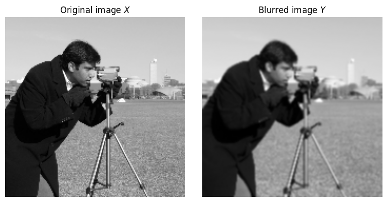

We can rewrite the convolution as a linear operation (see also below) using the vectorization operator $\operatorname{vec}()$. Define $y = \operatorname{vec}(Y) \in \mathbb{R}^{HW}$, $x = \operatorname{vec}(X) \in \mathbb{R}^{HW}$ and $b = \operatorname{vec}(B) \in \mathbb{R}^{HW}$, the above observation model is rewritten as

where $A$ is the matrix representing convolution with $K$. The least squares problem is then:

For the above example, $A$ is a huge structured matrix of size $HW \times HW$. To simplify the presentation, assume $H = W = 10$ (the matrix $A$ is already $100 \times 100$!)

Source

import matplotlib.patches as patches

def build_convolution_matrix(kernel, image_shape):
    """
    Build a convolution matrix A such that:
    y_flat = A @ x_flat
    where x_flat is the flattened image, and kernel is the convolution filter.
    """
    H, W = image_shape
    kH, kW = kernel.shape
    pad_h, pad_w = kH // 2, kW // 2

    # Number of pixels
    N = H * W
    # Initialize the convolution matrix
    A = np.zeros((N, N))

    # Iterate over each pixel in the image
    for i in range(H):
        for j in range(W):
            row = i * W + j # Row index in A

            # Place kernel centered at (i,j)
            for m in range(kH):
                for n in range(kW):
                    ii = i + m - pad_h
                    jj = j + n - pad_w
                    if 0 <= ii < H and 0 <= jj < W:
                        col = ii * W + jj
                        A[row, col] = kernel[m, n]
    return A

image_shape = 10, 10
A = build_convolution_matrix(K, image_shape)


fig, ax = plt.subplots(figsize=(8,8))
im = ax.imshow(A, cmap='gray_r', interpolation='none')
plt.title("Full Convolution Matrix $A$")
plt.colorbar(im, ax=ax, fraction=0.046, pad=0.04)

# Inset: show top-left 2 blocks along each direction
block_size_x = image_shape[0]
block_size_y = image_shape[1]
inset_size = block_size_x + block_size_y

# Create inset axes
ax_inset = ax.inset_axes([0.6, 0.6, 0.35, 0.35])
ax_inset.imshow(A[:20, :20], cmap='gray_r', interpolation='none')
ax_inset.set_title('first two blocks of $A$')
plt.show()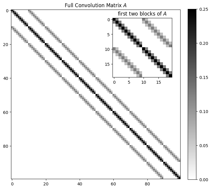

In practice, due to the large size of the matrix $A$, we do not use direct solutions based on pseudo-inverse calculations (see later on). In this case, the least squares problem is solved through the use of FFTs.

from numpy.fft import fft2, ifft2

# compute least squares solution using FFT
Y_fft = fft2(Y)
K_fft = fft2(K, s=X.shape)
eps = 1e-6*np.max(np.abs(K_fft))
X_hat = np.real(ifft2(Y_fft/(1+K_fft+eps))) # small epsilon for stability

# Display results
fig, axs = plt.subplots(1, 3, figsize=(10, 3))
axs[0].imshow(X, cmap='gray')
axs[0].set_title("True image $X$")
axs[1].imshow(Y, cmap='gray')
axs[1].set_title("Blurred observation $Y$")
axs[2].imshow(X_hat, cmap='gray')
axs[2].set_title("LS estimate $\hat{X}$")
for ax in axs: ax.axis('off')
plt.tight_layout()
plt.show()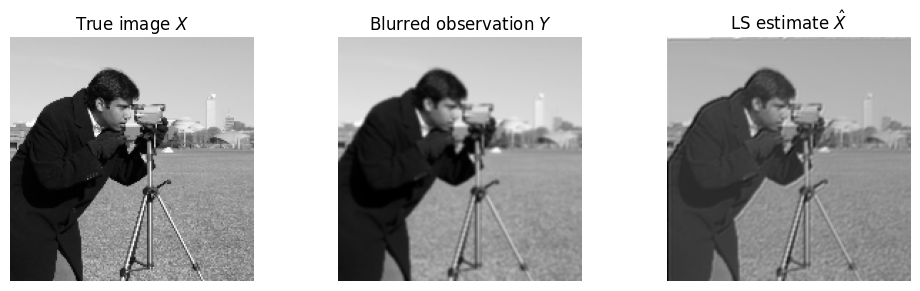

This example demonstrates how 2D deconvolution can be formulated and solved as a linear least squares problem.