3.1A first example: linear regression

Let us assume we are observing some data $y_1, y_2, \ldots, y_n$ as a function of a variable $x$ as depicted in the following plot:

Source

import numpy as np
import matplotlib.pyplot as plt

np.random.seed(2025)
beta0 = 1
beta1 = 1.5

n = 30
x = np.linspace(0, 10, n)
y = beta0 + beta1 * x + 1.2*np.random.randn(n)

plt.scatter(x, y, label="measurement $y_i$")
plt.xlabel(r"$x$")
plt.ylabel(r"$y$")
plt.ylim(0, 20)
plt.legend()
plt.show()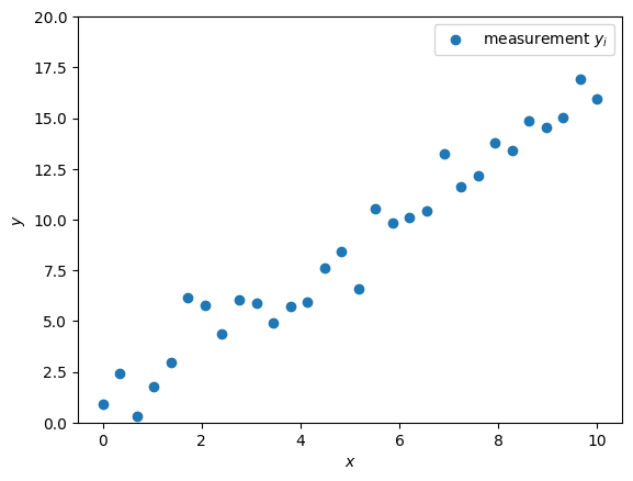

Formulating the optimization problem¶

Suppose we are interested in finding a straightforward mathematical relationship that links the input (or explanatory) variables $x_i$ to the observed data points $y_i$. In other words, we want to model how the measurements $y_i$ depend on the values of $x_i$. This process is known as regression analysis, and in this example, we will focus on linear regression, which assumes that the relationship between $x_i$ and $y_i$ can be well-approximated by a straight line, or in mathematical terms:

Let’s construct an objective function in the parameters $(\beta_0, \beta_1)$. A first simple choice is to measure the error (or residual) between the model and the observations using a quadratic function

leading to the total model error

For a fixed data vector $y = [y_1, \ldots, y_n]^\top$ and known explanatory variables $x = [x_1, \ldots, x_n]^\top$, we obtain the following unconstrained optimization problem in terms of $\beta = [\beta_0, \beta_1]^\top$:

This is a linear least squares problem. This type of problem is found in many applications, such as engineering, econometrics, image processing, etc.

Computing the solution¶

Linear regression is widely used across many fields, and there are numerous readily available tools for computing solutions. The goal of this chapter is to look under the hood of such tools. In the meantime, here’s how to solve the problem (4) using scikit-learn:

from sklearn.linear_model import LinearRegression

# Reshape x for scikit-learn
X = x.reshape(-1, 1)
model = LinearRegression()
model.fit(X, y)

# Extract coefficients
beta0_hat = model.intercept_
beta1_hat = model.coef_[0]

print(f"Estimated coefficients: beta0 = {beta0_hat:.2f}, beta1 = {beta1_hat:.2f}")
print(f"Ground truth coefficients: beta0 = {beta0:.2f}, beta1 = {beta1:.2f}")

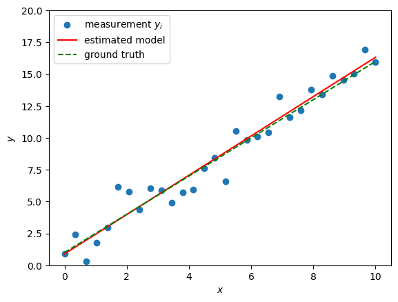
# Display the fitted line
plt.scatter(x, y, label="measurement $y_i$")
plt.plot(x, beta0_hat + beta1_hat * x, color="red", label="estimated model")
plt.plot(x, beta0 + beta1 * x, color="green", linestyle='--', label="ground truth")

plt.xlabel(r"$x$")
plt.ylabel(r"$y$")
plt.ylim(0, 20)
plt.legend()
plt.show()

Estimated coefficients: beta0 = 0.89, beta1 = 1.54
Ground truth coefficients: beta0 = 1.00, beta1 = 1.50