Local and global optima - Mines Nancy

Definitions¶

Consider the general constrained optimization problem

\begin{array}{ll} \minimize& f_0(x)\\ \st & x \in \Omega\end{array}

(1)

We suppose that the problem is solvable, i.e., $p^\star$ is finite and there exists $x^\star \in \Omega$ such that $f(x^\star) = p^\star$ . In many settings, it is important to be able to distinguish between local and global optima of a given optimization problem.

$x_1$ is a strict global optimum
$x_2$ is a strict local optimum
$x_3$ is a local optimum

Examples¶

To illustrate the notion of local / global optima we consider the unconstrained optimization case of a given function $f_0(x)$ .

1D polynomial function¶

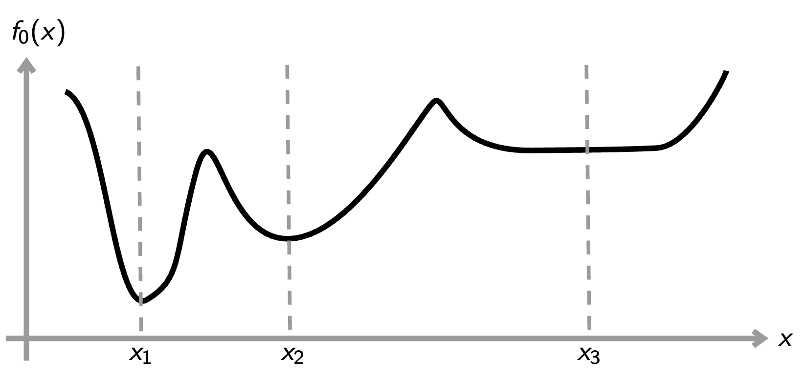
Consider the 1D function defined over $\mathbb{R}$ as

f_0(x) = 360x - 6x^2 - 498.167x^3 + 13.1875x^4 + 44x^5 - 3.20833x^6 - 1.14286x^7 + 0.125x^8

(3)

The unconstrained optimization problem, which consists in finding $x$ that minimizes $f_0$ over $\mathbb{R}$ , admits a unique solution given by $x^\star = 6$ (the global optimum). Yet they are many local optima, as shown by the following snippet.

import numpy as np
import matplotlib.pyplot as plt

def f(x):
    return (360*x - 6*x**2 - 498.167*x**3 + 13.1875*x**4 +
            44*x**5 - 3.20833*x**6 - 1.14286*x**7 + 0.125*x**8)

# Local optima
mins = np.array([-4, -0.5, 4, 6])

print("Values at local optima:")
for min_x in mins:
    print(f"x = {min_x}, f(x) = {f(min_x)}")

x = np.linspace(-4.5, 6.5, 100)
plt.plot(x, f(x), linewidth=2)
for min_x in mins[:-1]:
    l1 = plt.axvline(min_x, color="green", linestyle='--')
    l2 = plt.hlines(f(min_x), min_x-1, min_x+1, color="green", linestyle='-.')

l3 = plt.axvline(mins[-1], color="red", linestyle='--')
l4 = plt.hlines(f(mins[-1]), mins[-1]-1, mins[-1]+1, color="red", linestyle='-.')
plt.xlabel(r"$x$")
plt.ylabel(r"$f_0(x)$")
plt.legend([l1, l2, l3, l4], ['local optimum', 'local optimum value', 'global optimuù', 'global optimum value'], loc=1)
plt.show()

Values at local optima:
x = -4.0, f(x) = 2441.986559999994
x = -0.5, f(x) = -119.82061953125002
x = 4.0, f(x) = -5780.625919999999
x = 6.0, f(x) = -6088.573439999978

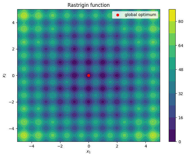
2D function¶

The Rastrigin function is a non-convex function commonly used as a performance test problem for optimization algorithms. Its expression in two dimensions is given by:

f_0(x_1, x_2) = 20 + x_1^2 + x_2^2 - 10\left(\cos(2\pi x_1) + \cos(2\pi x_2)\right)

(4)

where $x_1, x_2 \in \mathbb{R}$ . As shown by the following code snippet, it has many local optima and a single global optimum at $(x_1, x_2) = (0, 0)$ .

import numpy as np
import matplotlib.pyplot as plt
def f(x1, x2):
    return 20 + x1**2 + x2**2 - 10 * (np.cos(2 * np.pi * x1) + np.cos(2 * np.pi * x2))

x1s = np.linspace(-5, 5, 100)
x2s = np.linspace(-5, 5, 100)
X1, X2 = np.meshgrid(x1s, x2s)
Z = f(X1, X2)

plt.figure(figsize=(8, 6))
contour = plt.contourf(X1, X2, Z, levels=10)
plt.scatter([0], [0], color='red', label='global optimum')
plt.xlabel("$x_1$")
plt.ylabel("$x_2$")
plt.title("Rastrigin function")
plt.colorbar(contour)
plt.legend()
plt.show()

Mines Nancy - Optimization course

Continuous optimization problems: general form