1.1Introductory example

Problem statement¶

To motivate first definitions, let us consider the following practical shape optimization problem.

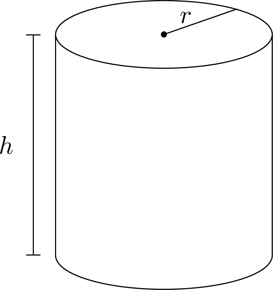
A can producer wants to optimize his consumption of raw material.

They formulate one explicit constraint: the volume of the can must be $V_0 = 1$ L.

We assume objects of constant thickness $e$. Therefore, the quantity of raw material is simply given by

Since the goal is to optimize (i.e., in this case, minimize) the consumption of raw material, the optimization problems can be formulated in layman’s terms as follows:

Mathematical formulation¶

Expression of the area $A$ (objective function or criterion)

The dimensions $r$ and $h$ are the variables of the optimization problem.

Constraints We have explicit and implicit constraints:

• Constant volume $V_0 = 1$ L. This one is explicitly given in the statement of the problem, and reads
  $$V(r, h) = \pi r^2 h = V_0$$

  (3)
• Non-negativity: the variables $r$ and $h$ must be non-negative owing to their interpretation as physical dimensions
  $$r\geq 0,\qquad h\geq 0$$

  (4)

The constrained optimization problem is finally written as

Simplification¶

Notice that $h$ and $r$ are related by the constraint $V_0 = \pi r^2 h$. Therefore, the area $A(r, h)$ can be rewritten as a function of $r$ only. Using

and substituting this into the expression for $A(r, h)$, one obtains

The volume constraint is directly taken into account in the new objective function $\tilde{A}(r)$. We consider the constraint $r\geq 0$ when searching for the minimum of $\tilde{A}(r)$ over $\mathbb{R}_+$;

Visualization using Python¶

Let us plot the objective function using basic Python commands.

# import libraries
import numpy as np # for manipulation of arrays
import matplotlib.pyplot as plt # for plotting

# function definitions
def h(r, V0=1000):
    return V0 / (np.pi * r**2)

def A_lids(r):
    return 2 * np.pi * r**2

def A_cylinder(r):
    return 2 * np.pi * r * h(r)

def A(r):
    return A_couvercle(r) + A_cylindre(r)

# define variables and constraints
V0 = 1000  # volume in cm^3 (=1 L)
r = np.linspace(1, 15, 100)  # vector of 100 values linearly spaced between 1 and 15

# do the plotting
plt.plot(r, A_lids(r), label="lids area", linewidth=2, linestyle='--')
plt.plot(r, A_cylinder(r), label="cylinder area", linewidth=2, linestyle=':')
plt.plot(r, A_lids(r) + A_cylinder(r), label="total area", linewidth=2)
plt.xlabel("radius r [cm]")
plt.ylabel("objective value [cm^2]")
plt.legend()
plt.show()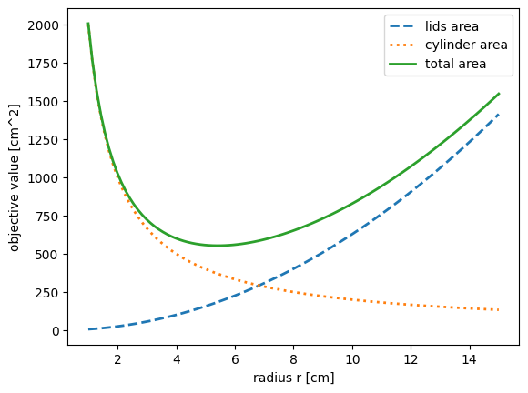

The plot suggests a minimizer exists, somewhere between $r=4$ cm and $r = 6$ cm. Quite naturally, the minimum area value is obtained when the derivative of $\tilde{A}(r)$ vanishes. Let us do the explicit computation.

Explicit solutions¶

The derivative of the objective function vanishes at its minimum.

We solve

In summary, the solutions to the optimization problem are

We can also check that our computations are correct using Python, by modifying the previous code.

# optimal value
r_star= (V0/(2*np.pi))**(1/3)

# do the plotting
plt.plot(r, A_lids(r), label="lids area", linewidth=2, linestyle='--')
plt.plot(r, A_cylinder(r), label="cylinder area", linewidth=2, linestyle=':')
plt.plot(r, A_lids(r) + A_cylinder(r), label="total area", linewidth=2)
plt.axvline(r_star, label="optimal radius", linewidth=2, color="black")
plt.axhline(A_lids(r_star) + A_cylinder(r_star), label="optimal area", linewidth=2, color="black", linestyle='--')
plt.xlabel("radius r [cm]")
plt.ylabel("objective value [cm^2]")
plt.legend()
plt.show()

print(f"Optimal value of r minimizing A(r): r_opt = {r_star:.2f} cm")
print(f"Minimal area A(r_opt): A_min = {A_lids(r_star) + A_cylinder(r_star):.2f} cm^2")
print(f"Associated optimal height value h(r_opt): h_opt = {h(r_star):.2f} cm")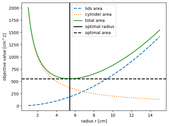

Optimal value of r minimizing A(r): r_opt = 5.42 cm
Minimal area A(r_opt): A_min = 553.58 cm^2
Associated optimal height value h(r_opt): h_opt = 10.84 cm

You can play around with this code snippets and see how the solution changes as we modify the value of $V_0$.