4.7Choosing an algorithm: convergence rates and computational cost tradeoffs

Consider the optimization problem

and assume a solution exists, i.e., there exists $x^\star \in \mathbb{R}^n$ such that $f(x^\star) = p^\star < \infty$. The choice of an algorithm for solving the problem usually depends on a tradeoff between two essential properties:

• Convergence rate: It indicates how fast the iterates approach their limit, measured e.g., using

  • $\varepsilon_k = \vert f(x^{(k)}) - p^\star\vert$ (convergence in objective values)

  • $\varepsilon_k = \Vert x^{(k)} - x^\star\Vert_2$ (convergence in iterates)

  The rate of convergence is asymptotic, meaning it appears as $k \rightarrow \infty$.

• Numerical complexity: It measures the computational cost associated with an algorithm (usually, the cost per iteration).

Typical convergence rates¶

Depending on how the metric $\varepsilon_k$ behaves asymptotically, we define several convergence rates:

• Linear convergence:
  $$\frac{\varepsilon_{k+1}}{\varepsilon_k} \underset{k\rightarrow \infty}{\rightarrow} \mu, \quad 0 < \mu < 1$$

  (2)
• Super-linear convergence:
  $$\frac{\varepsilon_{k+1}}{\varepsilon_k} \underset{k\rightarrow \infty}{\rightarrow} 0$$

  (3)
• Quadratic convergence:

The terms linear, superlinear and quadratic refer to the curves made by the metric $\varepsilon_k$ across iterations, in a semilogy plot, as shown below.

Source

import numpy as np
import matplotlib.pyplot as plt

iters = np.arange(0, 50)
eps0 = 1
rate=.95
linear = eps0 * rate ** iters
superlinear = eps0 * rate ** (iters ** 1.5)
quadratic = eps0 * rate ** (2 ** iters)
quadratic[10:] = 0
plt.semilogy(iters, linear, 'o-', label='Linear')
plt.semilogy(iters, superlinear, 's-', label='Superlinear')
plt.semilogy(iters, quadratic, '^-', label='Quadratic')
plt.xlabel('Iteration')
plt.ylabel('Error metric')
plt.legend()
plt.title('Convergence Rates')
plt.show()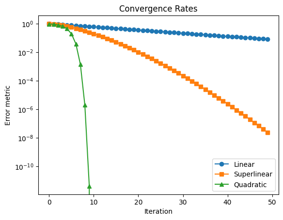

Computational complexity¶

The computational complexity of an algorithm is often measured in terms of flops (floating-point operations), which count the number of basic arithmetic operations such as addition and multiplication.

The table below summarizes the complexity of some basic operations.

Note these are complexity obtained by standard, simple implementations; some complexities can be refined in some settings by taking into account the structure (sparsity, etc.) of matrices and vectors.

The total computational cost of an algorithm depends on the sequence and combination of such operations. In practice, other factors like memory usage and data movement can also significantly affect performance.

Properties of some classical algorithms¶

More to come in the dedicated chapter on convergence properties. These results apply to unconstrained problems (for constrained problems, some of these results hold under certain conditions).

• Gradient method with constant step size

  $$x^{(k+1)} = x^{(k)} - \alpha \nabla f_0(x^{(k)})$$

  (5)

  • Complexity: $\mathcal{O}(n)$ per iteration

  • Linear convergence rate [under some conditions]

• Newton’s method

• Complexity: $\mathcal{O}(n^3)$ per iteration
• Quadratic convergence rate [under some conditions]