Time-Frequency-Polarization analysis: tutorial
This tutorial aims at demonstrating different tools available within the
timefrequency module of BiSPy. The examples provided here come
along with the paper
Julien Flamant, Nicolas Le Bihan, Pierre Chainais: “Time-frequency analysis of bivariate signals”, In press, Applied and Computational Harmonic Analysis, 2017; arXiv:1609.0246, doi:10.1016/j.acha.2017.05.007.
The paper contains theoretical results and several applications that can be reproduced with the following tutorial. A Jupyter notebook version can be downloaded here.
Load bispy and necessary modules
import numpy as np
import matplotlib.pyplot as plt
import quaternion  # load the quaternion module
import bispy as bsp
Quaternion Short-Term Fourier Transform (Q-STFT) example
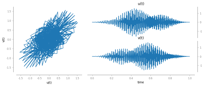
To illustrate the behaviour of the Q-STFT, we construct a simple signal made of two linear chirps, each having its own instantaneous polarization properties.
First, define some constants:
N = 1024 # length of the signal

# linear chirps constants
a = 250*np.pi
b = 50*np.pi
c = 150*np.pi
Then define the instantaneous amplitudes, orientation, ellipticity and phase of each linear chirp. The amplitudes are taken equal - just a Hanning window.
# time vector
t = np.linspace(0, 1, N)

# first chirp
theta1 = np.pi/4 # constant orientation
chi1 = np.pi/6-t # reversing ellipticity
phi1 = b*t+a*t**2 # linear chirp

# second chirp
theta2 = np.pi/4*10*t # rotating orientation
chi2 = 0 # constant null ellipticity
phi2 = c*t+a*t**2 # linear chirp

# common amplitude -- simply a window
env = bsp.utils.windows.hanning(N)
We can now construct the two components and sum it. To do so, we use the
function signals.bivariateAMFM to compute directly the quaternion
embeddings of each linear chirp.
# define chirps x1 and x2
x1 = bsp.signals.bivariateAMFM(env, theta1, chi1, phi1)
x2 = bsp.signals.bivariateAMFM(env, theta2, chi2, phi2)

# sum it
x = x1 + x2
Let us have a look at the signal x[t]
fig, ax = bsp.utils.visual.plot2D(t, x)
Now we can compute the Q-STFT. First initialize the object Q-STFT
S = bsp.timefrequency.QSTFT(x, t)
And compute:
S.compute(window='hamming', nperseg=101, noverlap=100, nfft=N)
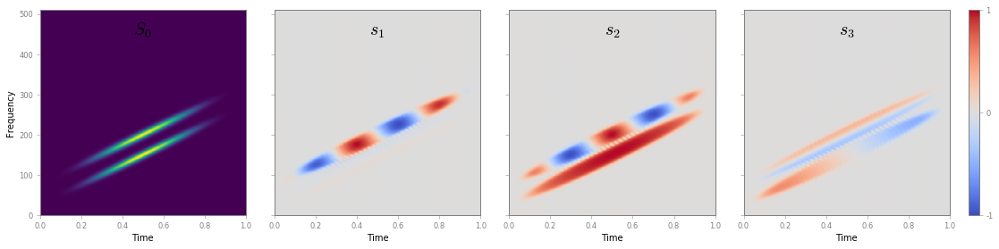
Computing Time-Frequency Stokes parameters
Let us have a look at Time-Frequency Stokes parameters S1, S2 and S3
fig, ax = S.plotStokes()
Alternatively, we can compute the instantaneous polarization properties from the ridges of the Q-STFT.
Extract the ridges:
S.extractRidges()
Extracting ridges
Ridge added
Ridge added
2 ridges were recovered.
And plot (quivertdecim controls the time-decimation of the quiver
plot, for a cleaner view):
fig, ax = S.plotRidges(quivertdecim=30)
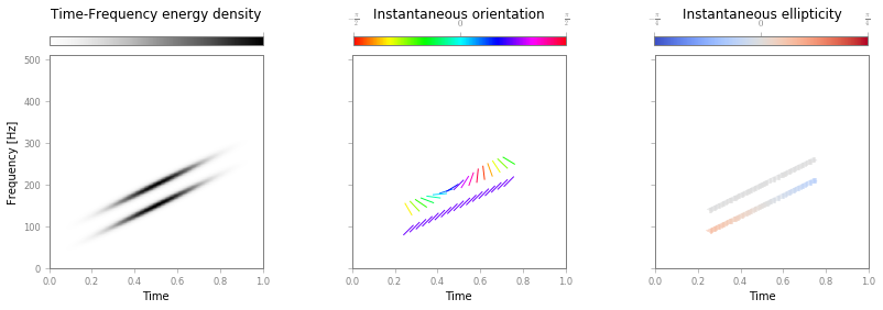
The two representations are equivalent and provide the same information: time, frequency and polarization properties of the bivariate signal. A direct inspection shows that instantaneous parameters of each components are recovered by both representations.
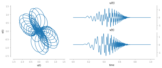
Quaternion Continuous Wavelet Transform (Q-CWT) example
The Q-STFT method has the same limitations as the usual STFT, that is not the ideal tool to analyze signals spanning a wide range of frequencies over short time scales. We revisit here the classic two chirps example in its bivariate (polarized) version.
As before, let us first define some constants:
N = 1024 # length of the signal

# hyperbolic chirps parameters
alpha = 15*np.pi
beta = 5*np.pi
tup = 0.8 # set blow-up time value
Now, let us define the instantaneous amplitudes, orientation, ellipticity and phase of each linear chirp. The chirps are also windowed.
t = np.linspace(0, 1, N) # time vector

# chirp 1 parameters
theta1 = -np.pi/3 # constant orientation
chi1 = np.pi/6 # constant ellipticity
phi1 = alpha/(.8-t) # hyperbolic chirp

# chirp 2 parameters
theta2 = 5*t # rotating orientation
chi2 = -np.pi/10 # constant ellipticity
phi2 = beta/(.8-t) # hyperbolic chirp

# envelope
env = np.zeros(N)
Nmin = int(0.1*N) # minimum value of N such that x is nonzero
Nmax = int(0.75*N) # maximum value of N such that x is nonzero

env[Nmin:Nmax] = bsp.utils.windows.hanning(Nmax-Nmin)
Construct the two components and sum it. Again we use the function
utils.bivariateAMFM to compute directly the quaternion embeddings of
each linear chirp.
x1  = bsp.signals.bivariateAMFM(env, theta1, chi1, phi1)
x2  = bsp.signals.bivariateAMFM(env, theta2, chi2, phi2)

x = x1 + x2
Let us visualize the resulting signal, x[t]
fig, ax = bsp.utils.visual.plot2D(t, x)
Now, we can compute its Q-CWT. First define the wavelet parameters and initialize the QCWT object:
waveletParams = dict(type='Morse', beta=12, gamma=3)
S = bsp.timefrequency.QCWT(x, t)
And compute:
fmin = 0.01
fmax = 400
S.compute(fmin, fmax, waveletParams, N)
Computing Time-Frequency Stokes parameters
Let us have a look at Time-Scale Stokes parameters S1, S2 and S3
fig, ax = S.plotStokes()
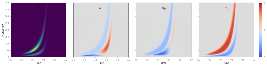
Similarly we can compute the instantaneous polarization attributes from the ridges of the Q-CWT.
S.extractRidges()
Extracting ridges
Ridge added
Ridge added
2 ridges were recovered.
And plot the results
fig, ax = S.plotRidges(quivertdecim=40)
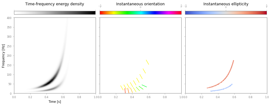
Again, both representations are equivalent and provide the same information: time, scale and polarization properties of the bivariate signal. A direct inspection shows that instantaneous parameters of each components are recovered by both representations.